Lecture 20 - Heterodyne Radios
EE-30023/31023, Department of Electrical Engineering, University of Notre Dame
Summary
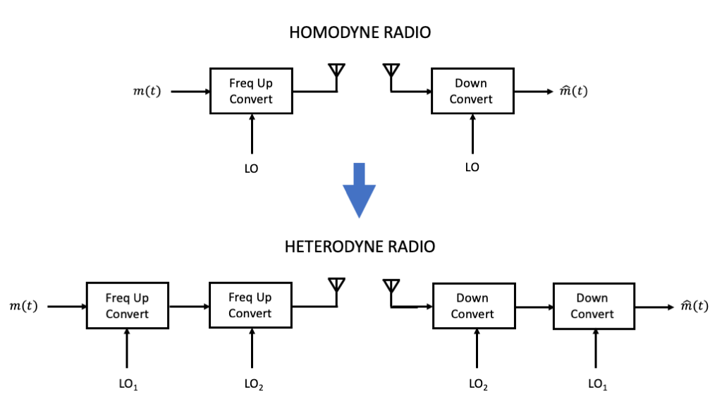
In this lecture, we will address some of the limitations of homodyne radios by adding stages of frequency upconversion in the transmitter and downconversion in the receiver. Such techniques lead to heterodyne radios, and provide additional flexibility in order to improve radio performance.
Motivation in Course Context
In the previous week of lecture and lab, we studied various techniques from upconverting a baseband signal to a passband carrier frequency, and correspondingly downconverting a passband signal back to baseband. Frequency up- and down-conversion were each performed in one step, which is called homodyning.
By contrast, in this lecture, we will develop conceptual understanding and practical system design guidelines for performing frequency up- and down-conversion in multiple steps, which is called heterodyning.
These two approaches are illustrated in the figure below.
Terminology
Defintion: An intermediate frequency (IF) is a positive frequency aside from the carrier frequency that is used as part of the transmitter modulation or receiver modulation process.
Definition: Using one (or more) intermediate frequencies as part of a transmit or receive chain is called heterodyning.
Definition: Using no intermediate frequencies as part of a transmit or receive chain is called homodyning. Another recently-used term for such techniques is direct conversion.
Heterodyne Concepts
Let \(s_i(t)\) be a signal of passband bandwidth at most \(2B\), \(B > 0\), at the intermediate frequency \(f_i > B\).
For generality, we will consider that \(s_i(t)\) is generated from quadrature multiplexing of two real-valued baseband signals \(m_1(t)\) and \(m_2(t)\), each with baseband bandwidth \(B\), according to
\[ s_i(t) = m_1(t)\cos(2\pi f_i t) - m_2(t)\sin(2\pi f_i t) \]
Recall that:
For DSB-SC, \(m_2(t)=0\)
For SSB, \(m_2(t)\) is the positive or negative Hilbert transform of \(m_1(t)\), and the passband bandwidth is only \(B\).
Otherwise, we can view the modulation scheme as inputting a complex-valued baseband signal \(m(t)=m_1(t)+j m_2(t)\) and creating
\[ s_i(t) = \mathrm{Re}\left\{ m(t) e^{j2\pi f_i t} \right\} \]
IF to Carrier Passband Conversion
If we modulate \(s_i(t)\) with another sinusoidal oscillator signal of frequency \(f_{o} > f_{i}\), we have
\[\begin{align} s_i(t) \cos(2\pi f_o t + \vartheta) =& m_1(t)\cos(2\pi f_i t)\cos(2\pi f_o t + \vartheta) - m_2(t)\sin(2\pi f_i t)\cos(2\pi f_o t + \vartheta) \\ =& \frac{1}{2} m_1(t)\left[\cos(2\pi (f_o+f_i) t + \vartheta) + \cos(2\pi (f_o-f_i) t + \vartheta) \right] \\ &- \frac{1}{2} m_2(t) \left[ \sin(2\pi (f_o+f_i) t + \vartheta) + \sin(2\pi (f_o-f_i) t + \vartheta)\right] \\ =& \frac{1}{2}\left\{ m_1(t)\cos(2\pi (f_o+f_i) t + \vartheta) - m_2(t)\sin(2\pi (f_o+f_i) t + \vartheta )\right\} \\ & + \frac{1}{2} \left\{ m_1(t)\cos(2\pi (f_o-f_i) t + \vartheta) - m_2(t)\sin(2\pi (f_o-f_i) t + \vartheta \right\} \\ =& \frac{1}{2} \mathrm{Re}\left\{ m(t) e^{j2\pi (f_o+f_i) t} \right\} + \frac{1}{2} \mathrm{Re}\left\{ m(t) e^{j2\pi (f_o-f_i) t} \right\} \end{align}\]
where we have applied the trigonometric identities \(\cos(A)\cos(B)=\frac{1}{2}[\cos(A+B)+\cos(A-B)]\) and \(\sin(A)\cos(B)=\frac{1}{2}[\sin(A+B)+\sin(A-B)]\).
From the final representation, we see that the multiplication has produced two passband components at frequencies \(f_o+f_i\) and \(f_o - f_i\), respectively, as illustrated for positive frequencies in the figure below.
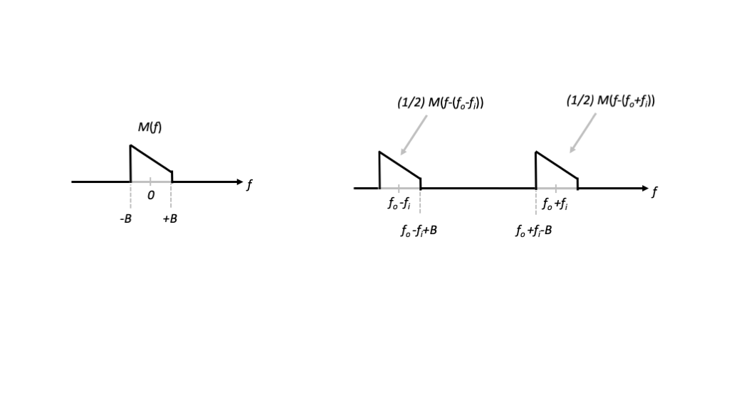
Note that we have intentionally drawn \(M(f)\) to be asymmetric at baseband, to clearly suggest that it represents a complex-valued baseband waveform.
This immediately leads to two ways of generating a passband signal at a desired carrier frequency \(f_c\).
Subheterodyne Conversion
First, we can set \(f_o=f_c-f_i\), so that the oscillator frequency is below the desired carrier frequency. This is referred to as subheterodyne conversion. In this case, \(f_c = f_o + f_i\), and we want to maintain the frequency content centered at the sum of the oscillator and intermediate frequencies. We therefore bandpass filter the output at the frequency \(f_c\) so that the frequency content centered at \(f_o - f_i\) is eliminated.
This downconversion process is summarized in the figure below.

In this case, the output signal at the carrier frequency satisfies
\[\begin{align} s_c(t) =& m_1(t)\cos(2\pi f_c t + \vartheta) - m_2(t)\sin(2\pi f_c t + \vartheta) \\ =&\mathrm{Re}\left\{ m(t) e^{j2\pi f_c t + \vartheta} \right\} \end{align}\]
Superheterodyne Conversion
Second, we can set \(f_o=f_c+f_i\), so that the oscillator frequency is above the desired carrier frequency. This is referred to as superheterodyne conversion. In this case, \(f_c = f_o - f_i\), and we want to maintain the frequency content centered at the difference of the oscillator and intermediate frequencies. We again bandpass filter the output at the frequency \(f_c\) so that the frequency content centered at \(f_o + f_i\) is eliminated.
This downconversion process is summarized in the figure below.

Again, the output signal at the carrier frequency satisfies
\[\begin{align} s_c(t) =& m_1(t)\cos(2\pi f_c t + \vartheta) - m_2(t)\sin(2\pi f_c t + \vartheta) \\ =&\mathrm{Re}\left\{ m(t) e^{j2\pi f_c t} \right\} \end{align}\]
From this development, we see that the second stage of upconversion, whether we use the sub- or super-heterodyne approach, gives us the same result. Furthermore, the result is mathematically equivalent direct converstion from baseband directly to the desired carrier frequency.
Carrier to IF Passband Conversion
Now let \(s_c(t)\) be a signal of passband bandwidth at most \(2B\), \(B > 0\), at the carrier frequency \(f_c\). And suppose that we wish to convert this signal to be at an intermediate frequency \(f_i\) such that \(f_c > f_i > B\).
Again, we consider \(s_c(t)\) to be of the form
\[ s_c(t)=m_1(t)\cos(2\pi f_c t) - m_2(t)\sin(2\pi f_c t) = 2\mathrm{Re}\left\{m(t) e^{j2\pi f_c t} \right\} \]
for some baseband signal \(m(t)\) for generality.
If we modulate \(s_c(t)\) with a sinusoidal oscillator signal of frequency \(f_o < f_c\), we have
\[\begin{align} s_c(t) \cos(2\pi f_o t + \vartheta) =& m_1(t)\cos(2\pi f_c t)\cos(2\pi f_o t + \vartheta) - m_2(t)\sin(2\pi f_c t)\cos(2\pi f_o t + \vartheta) \\ =& \frac{1}{2} m_1(t)\left[\cos(2\pi (f_c+f_o) t + \vartheta) + \cos(2\pi (f_c-f_o) t + \vartheta) \right] \\ &- \frac{1}{2} m_2(t) \left[ \sin(2\pi (f_c+f_o) t + \vartheta) + \sin(2\pi (f_c-f_o) t + \vartheta)\right] \\ =& \frac{1}{2}\left\{ m_1(t)\cos(2\pi (f_c+f_o) t + \vartheta) - m_2(t)\sin(2\pi (f_c+f_o) t + \vartheta )\right\} \\ & + \frac{1}{2}\left\{ m_1(t)\cos(2\pi (f_c-f_o) t + \vartheta) - m_2(t)\sin(2\pi (f_c-f_o) t + \vartheta \right\} \\ =& \frac{1}{2}\mathrm{Re}\left\{ m(t) e^{j2\pi (f_c+f_o) t} \right\} + \frac{1}{2} \mathrm{Re}\left\{ m(t) e^{j2\pi (f_c-f_o) t} \right\} \end{align}\]
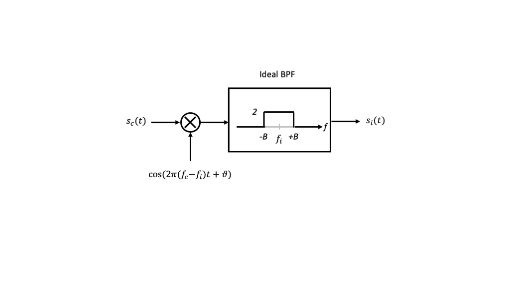
Although this in principle leads to two ways to translate the frequency content to a target intermediate frequency \(f_i\), typically we set the oscillator frequency \(f_o = f_c-f_i\) and we bandpass filter the output centered at \(f_i\), so that the frequency content centered at \(f_c+f_o\) is eliminated.
This downconversion process is summarized in the figure below.
Circuit Issues
Reduced Impact of LO Leakage and DC Offset
Recalling the implementation of the up- or down-conversions above via oscillators and mixers, we can now see how the carrier leakage and DC offsets can be reduced.
First, in the transmitter upconversion process, we were particularly concerned about LO leakage. For subheterodyne conversion, the leaked LO is at frequency \(f_c - f_i\), but we have a bandpass filter centered at \(f_c\). As long as \(f_c - f_i \ll f_c - B\), the filter will significantly eliminate the LO leakage. This corresponds to having a reasonably large \(f_i \gg B\).
Second, in the receiver downconversion process, we were particularly concerned about DC offset. Provided \(f_i - B \gg 0\), this DC offet will be heavily filtered by the bandpass filter above. So again, this suggests using a relatively large intermediate frequency \(f_i \gg B\).
In either aspect, the larger the intermediate frequency, the more flexibility we have in the transition band width and the stopband attenuations for the filters, giving us a great degree of flexibility in our radio designs.
Circuits at IF Often Better Performing
For tunability, we can allow the target carrier frequency \(f_c\) variable and fixe \(f_i\). This allows for much more precise design of the circuits at \(f_i\). In particular, the filters with center frequency \(f_i\) can be designed to be very selective.
Multiple Stages
Can cascade more than one intermediate frequency stage, so that we can have double heterodyne conversion, triple heterodyne conversion, and so forth.
More Non-Linearities
Despite these benefits, we have to keep track of additional harmonics in heterodyne radios, which we address in the next lecture.
The Image Problem
We saw that in basic heterodyne upconversion, we needed to add a bandpass filter to select one of two passband components. It turns out that we need to add bandpass filtering as the first step of the downconversion process as well, to avoid the so-called image problem.
Consider the signal \(s(t)=\cos(2\pi f t)\), where we will treat \(f\) as variable, applied to the input of the first stage of the downconversion mixer shown in the figure below.
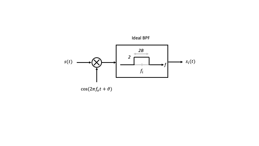
From our prior development with trigonometric identities, we know that the input to the filter will be the sum and difference signals
\[ s(t)\cos(2\pi f_o t + \vartheta) = \frac{1}{2}\left[\cos(2\pi (f_o+f) t + \vartheta) + \cos(2\pi (f_o-f) t + \vartheta)\right] \]
The figure below shows how the convolutions in the frequency domain can create frequency components in the positive frequency interval \([f_i-B,f_i+B]\) and negative frequency interval \([-f_i-B,-f_i+B]\).
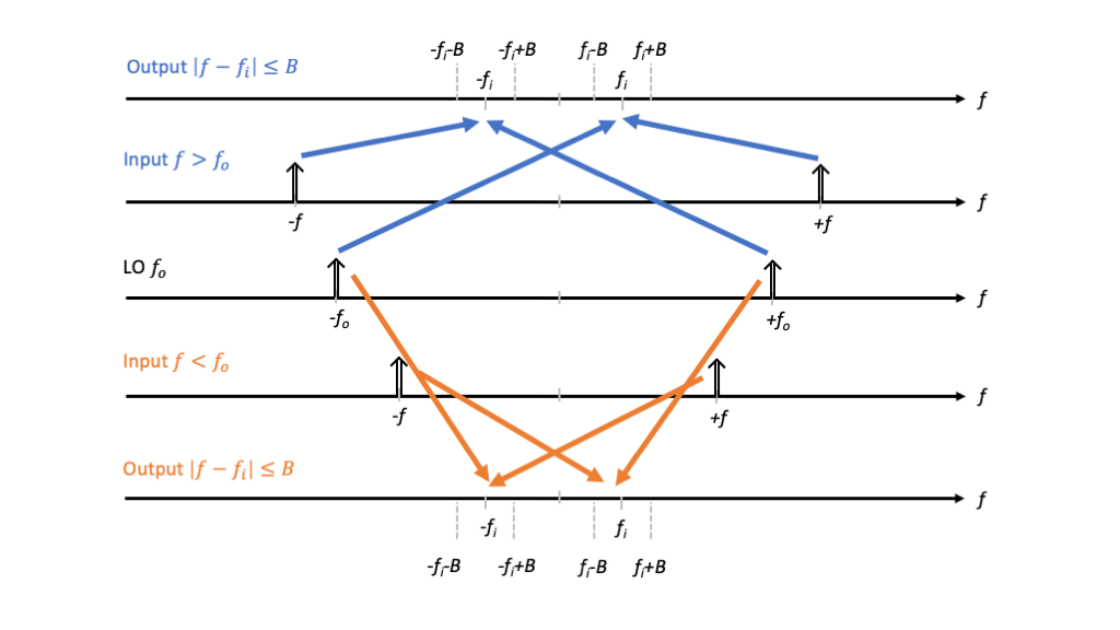
Specifically, for the case \(f > f_o\) (blue), we find that the bandpass filter passes any frequency satisfying
\[ f_i - B < f-f_o < f_i+B \]
or \(|f-(f_o+f_i)| < B\), which is the passband centered at \(f_o + f_i\) of bandwidth \(2B\).
Similary , for the case \(f < f_o\) (orange), we find that the bandpass filter passes any frequency satisfying
\[ f_i -B < f_o - f < f_i+B \]
or \(|f-(f_o-f_i)| < B\), which is the passband centered at \(f_o-f_i\) of bandwidth \(2B\).
These frequency bands are called the two image bands for the fixed mixer and IF bandpass filter, and are illustrated in the figure below.
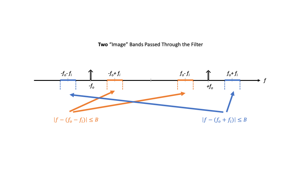
Given the above analysis, we observe that if our desired transmit signal’s frequency content is one of the heterodyne downconverter’s image bands, e.g., centered at \(f_o+f_i\), then the receiver will be susceptible to interference in the other frequency band, e.g., \(f_o - f_i\).
Image Reject Filtering
To reduce the impact of undesired images, we can add another bandpass filter at the input to the mixer. This additional filter is called an image reject filter.
This updated “ideal” downconverter architecture is shown in the figure below.
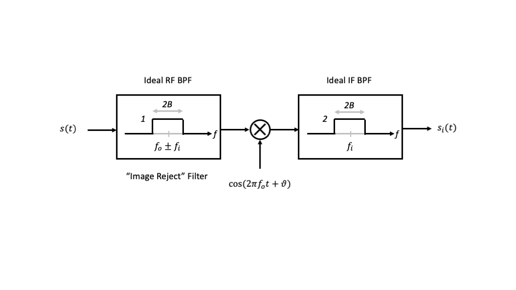
For clarity, the image reject filter selects either the image centered at \(f_o+f_i\) or \(f_o-f_i\), and is intended to reject the other.
The bandpass filters above are shown to have their passband including just the desired signal’s passband, and completely rejecting everything else. In practice, neither bandpass filter can be ideal, but will have a finite transition band and limited stopbband attenuation.
The figure below illustrates constraints on the RF bandpass filter if we intend to select inputs centered at \(f_o+f_i\) and reject inputs centered at \(f_o - f_i\).
In particular, we want the image reject filter to have significant attenuation at the frequency \(f_o-f_i + B\). If \(B\) and \(f_o\) are fixed, then we can relax the complexity and cost of the bandpass filter by selecting the intermediate frequency \(f_i\) as large as possible.
However, there may be practical constraints on the intermediate frequency as well. For example, we require \(f_i > B\) to ensure the first stage of modulation to the intermediate frequency does not have overlap in the frequency domain. There may also be an upper limit on the intermediate frequency imposed by the capabilities of the first mixing stage. The following example illustrates this point.
Example: Very often an intermediate frequency signal is generated in the transmitter and processed in the receiver using DT processing. If the minimum bandwidth of the DAC and ADC is denoted by \(W\ \mathrm{Hz}\) and we use NRZ signaling with bit rate and mainlobe bandwidth \(R=1/T\), then what is the largest possible IF frequency that should be allowed?
Answer: \(f_i < W - 1/T\). In fact, to ensure \(K-1\) sidelobes around the mainlobe, we would require \(f_i < W - K/T\).
Image Reject Mixing
Just as we saw that we could employ the Hilbert Transform and single sideband techniques to eliminate one sideband in homodyne upconversions, similar ideas can be applied to reject the undesired image in heterodyne downconversion. However, this approach requires Hilbert Transforms (implemented as \(\pi/2\) “hybrids”) and an additional mixer.
TBD: Expanded treatment