import numpy as np
import matplotlib.pyplot as pltLecture 08 - Link Performance
EE-30023/31023, Department of Electrical Engineering, University of Notre Dame
Summary
In this lecture, we will introduce several ways of characterizing and testing performance of a communication link regardless of the underlying physical medium and interface circuitry. Over time, we will connect these link layer performance metrics to physical layer parameters.
Motivation in Course Context
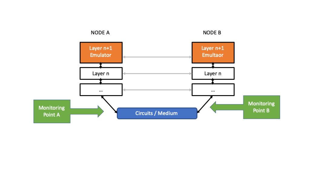
As we develop communication links and protocol layers above them, we will want to be able to characterize and test performance in a systematic way. This is summarized in the high-level block diagram in Figure 1.

As illustrated, we insert several additional elements into the layered protocols. These elements are often software components between higher layers, but they may be test and measurement hardware as we move closer to the physical medium. Two key elements that we insert for performance characterization and testing are:
Layer Emultators - software or hardware elements that generate valid packets for a given layer for input to the layer below, often based upon expected patterns and data rates. These packets can contain additional information to assist with the specific test being conducted, e.g., known bit patterns, timestamps, and so forth.
Monitoring Points - software or hardware elements that collect information at a specific point in the system, or between points in the system, in order to compute and report on performance measures, debugging information, and so forth
Outline
Measures
- Error Rates
- Throughput
- Delay
Measurement Tools
- iperf
- wireshark
Error Rates
Consider a sequence of payloads indexed by \(n=1,2,\ldots,N,\ldots\).
Let each payload be of length \(L_n\) bits, possibly changing with \(n\).
Let \(b_{l,n}\), \(l=1,2,\ldots,L_n\) denote the \(l\)-th bit of the \(n\)-th packet transmitted, and let \(\tilde{b}_{l,n}\) denote the corresponding received bit.
For convenience, we define the number of bit errors in packet \(n\) as \[ e_n := \sum_{l=1}^{L_n} | b_{l,n} - \tilde{b}_{l,n} | \]
Bit-Error Rate (BER)
The (empirical) bit-error rate (BER) is the quantity \[ \mathrm{BER}_N = \frac{\sum_{n=1}^{N} e_n }{\sum_{n=1}^{N} L_n} \tag{1}\]
Note that this quantity computes the total number of bit errors divided by the total number of bits transmitted in the \(N\) payloads.
If \(L_n = L\) for all payloads, then the denominator becomes \(NL\), and the BER simplifies to \[ \mathrm{BER}_N = \frac{1}{NL} \sum_{n=1}^{N} \sum_{l=1}^{L} |b_{l,n}-\tilde{b}_{l,n}| \tag{2}\]
Frame-Error Rate (FER)
The (empirical) frame-error rate (FER) is the quantity \[ \mathrm{FER}_N = \frac{1}{N} \sum_{n=1}^{N} \min(1,e_n) \tag{3}\]
Note that if there is any bit error in payload \(n\), then \(e_n \ge 1\), and it is counted in error in the summation. On the other hand, if there are no bit errors in payload \(n\), then \(e_n=0\), and it is not counted in error in the summation. Thus, this quantity represents the total number of payloads in error divided by the total number of transmitted payloads.
Often we consider performance for a very large number of payloads, and mathematically we take the limit as \(N \rightarrow \infty\). Since the empirial BER and FER can each be interpreted as the frequency of occurence of certain events, in many cases their limiting values can be analyzed using probability!
Example
Suppose a payload with integer length \(L\ge 1\) bits is subject to independent bit errors with probability \(0 \le p \le 1\).
- What is the probably of 2 or fewer bit errors in the payload?
Let \(E\) be the random variable representing the number of bit errors in the payload. \[\begin{align} \mathbb{P}[E \le 2] &= \mathbb{P}[E = 0] + \mathbb{P}[E = 1] + \mathbb{P}[E = 2] \\ &= (1-p)^L + \binom{L}{1} p (1-p)^{L-1} + \binom{L}{2}p^2(1-p)^{L-2} \end{align}\]
Here the sum results from mutual exclusivity of the events, and the powers of \(p\) and \((1-p)\) in each term result from the independences of the bit errors.
You may recognize that \(E\) has a binomial distribution, i.e., \(\mathbb{P}[E=l] = \binom{L}{l} p^l(1-p)^{L-l}\).
- What is the frame error probability?
A frame is in error if any of the bits are in error, i.e., the event \(E > 0\). \[ \mathbb{P}[E > 0] = 1-\mathbb{P}[E = 0] = 1 - (1-p)^L \]
- If we empirically measure \(\mathrm{BER}_N\) and \(\mathrm{FER}_N\) and let \(N \rightarrow \infty\), can we predict the result?
By the law of large numbers, we have \[ \lim_{N\rightarrow \infty} \mathrm{BER}_N = p \] and \[ \lim_{N\rightarrow \infty} \mathrm{FER}_N = 1 - (1-p)^L \]
And by the Central Limit Theorem, we can approximate \[ \mathrm{BER}_N \sim \mathbb{N}\left(p,\frac{p(1-p)}{NL}\right) \] where \(\mathbb{N}(\mu,\sigma^2)\) represents a Gaussian distribution with mean \(\mu\) and variance \(\sigma^2\).
Throughput
Consider again a sequence of payloads indexed by \(n=1,2,\ldots,N,\ldots\). Let each payload be of length \(L_n\) bits, possibly changing with \(n\).
Furthermore, let \(t_n\) denote the time that the payload passes a particular monitoring point in a system. The monitoring point could the input to a layer, or the output from a layer, for example.
The (empirical) throughput at a monitoring point over the interval \([0,T]\) is defined as the quantity \[ \mathrm{Throughput}_T = \frac{1}{T} \sum_{n: t_n \le T} L_n \tag{4}\]
That is, we count all the bits in the payloads that have passed the monitoring point before time \(T\), and we divde by \(T\).
Therefore the units of throughput will be bits per second.
As with error rates, we often consider very large time intervals, and mathematically we take the limit as \(T \rightarrow \infty\). The relevant probability theory is point processes, of which the Bernoulli and Poisson processes are particularly important.
Example
Suppose payloads cross a monitoring point according to a Poisson point process with rate \(\lambda\) per second. That is, during any time interval \([s_1,s_2)\), the number of payloads crossing is a Poisson random variable with mean \(\lambda(s_2 - s_1)\), and the number of payloads crossing in disjoint intervals are independent Poisson random variables.
If the average payload length is \(L\) bits, it can be shown that the empirical throughput satisfies \[ \lim_{T\rightarrow \infty} \mathrm{Throughput}_T = \lambda L \]
For completeness, recall that the random variable \(X\) has Poisson distribution with mean \(\gamma\) if \[ \mathbb{P}[X=k] = \frac{\gamma^k e^{-\gamma}}{k!}, \quad k=0,1,2,\ldots \]
Delay
Consider again a sequence of payloads indexed by \(n=1,2,\ldots,N,\ldots\). Here we want to characterize the amount of time it takes for payloads to move from one monitoring point to another monitoring point in a communication system.
Let time \(t_n\) denote the arrival time of payload \(n\) at the first monitoring point, and let \(s_n\) denote the departure time of payload \(n\) at the second monitoring point. The delay experienced by payload \(n\) is then \(d_n = s_n - t_n \ge 0\). We can also refer to \(d_n\) as the amount of time spent “in the system” between the two monitoring points.
The (empirical) delay between the two monitoring points is defined as the quantity \[ \mathrm{Delay}_N = \frac{1}{N} \sum_{n=1}^{N} d_n \tag{5}\]
Once again, we can obtain some insights about the system by considering average performance. We consider the average delay \(D = \lim_{N \rightarrow \infty} \mathrm{Delay}_N\), assuming the limit exists. The relevant probability theory is queuing theory and Markov processes.
Little’s Law
One important result, known as Little’s Law, states the following: If payloads arrive with rate \(\lambda\) at the first monitoring point, and spend on average \(D\) time in the system between the monitoring points, then the average number of payloads \(M\) in the system between the two monitoring points satisfies \[ M = \lambda D \tag{6}\]
Little’s Law applies in fairly general settings, and only requires that the system be stationary and stable. Stability in general requires that the service rate \(\mu\), which is the inverse of the average time required to process a single payload, be larger than the arrival rate \(\lambda\). If \(\mu < \lambda\), then the system will not be stable, and the number of payloads will grow unbounded.
Example
Suppose that payloads of length \(L\) bits arrival at a physical layer that adds a header of length \(H\) bits and transmits the packets at a rate of \(R\) bits per second.
- What is the service rate of this physical layer?
The service rate is the inverse of the average time required to transmit one packet. The total packet length is \(L+H\) bits, and therefore requires \((L+H)/R\) seconds for transmission. Thus, \(\mu = R/(L+H)\), with units of packets per second.
- What is the largest arrival rate of payloads to ensure stability?
\(\lambda < \mu = R/(L+H)\)
- What is the resulting throughput?
Measured at the input to the physical layer, the throughput will be \(\lambda L\), which must satisify \[ \lambda L < R \left( \frac{L}{L+H} \right) \]
Not surprisingly, the addition of the header bits in the physical layer reduces the maximum raw data rate \(R\) of the physical layer by the factor \(L/(L+H)\).
- Suppose packets arrive according to a Poisson process with rate \(\lambda\). What is the average number of packets in the system, and the average waiting time in the system?
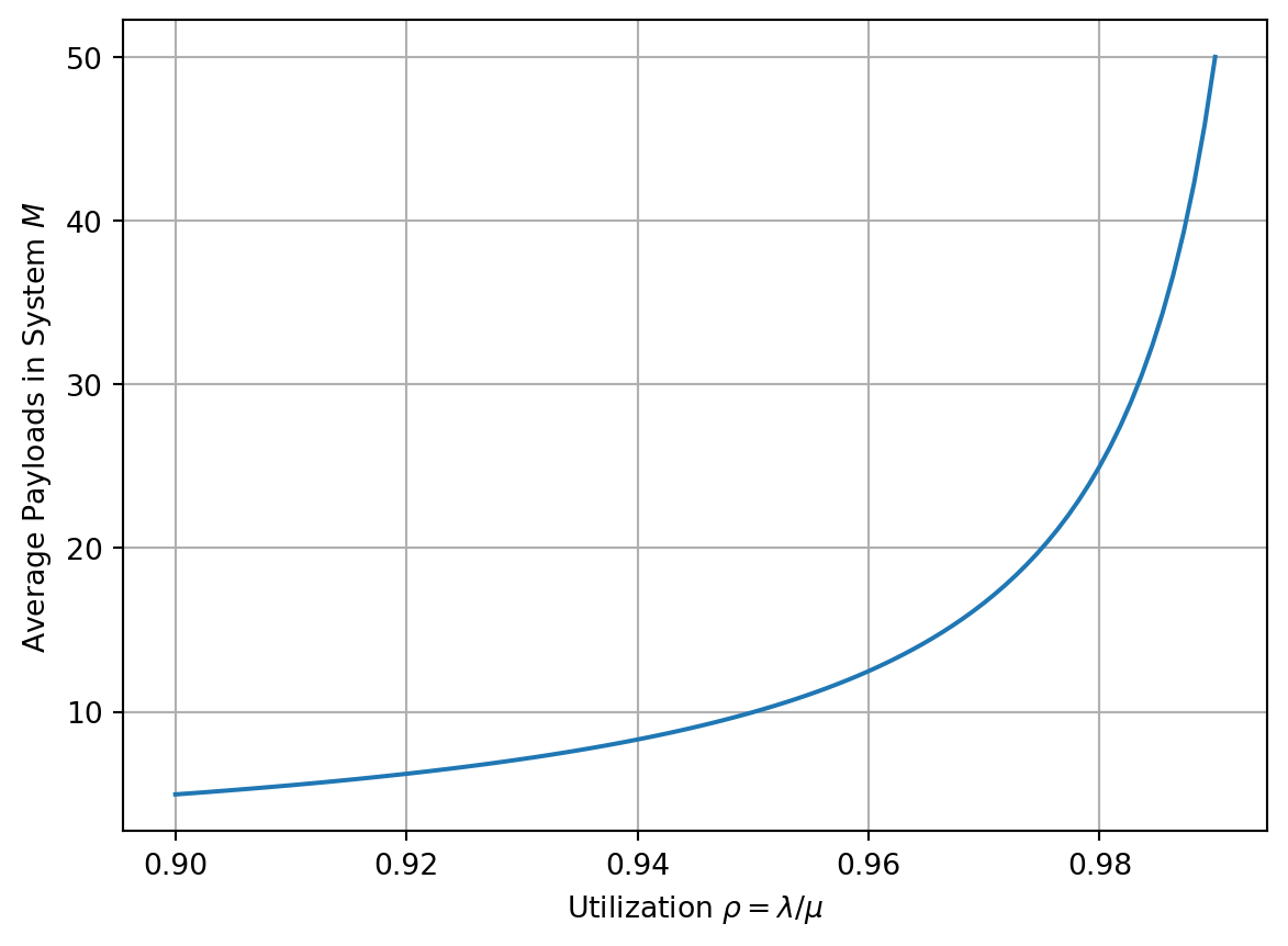
The M/D/1 queuing model (https://en.wikipedia.org/wiki/M/D/1_queue) can be applied to this system. The classic results are defined in terms of the utilization \(\rho = \lambda / \mu < 1\). Specifically, we have the average number of payloads in the system is \[ M=\rho + \frac{1}{2}\left( \frac{\rho^2}{1-\rho} \right) \] and the average waiting time in the system is \[ D=\frac{1}{\mu} + \frac{\rho}{2\mu(1-\rho)} \]
Notice that this system satisfies Little’s Law in that \(M=\lambda D\).
pts = 100
rho = np.linspace(0.9,1-1/pts,pts)
M = rho + rho**2/(1-rho)/2
plt.plot(rho,M,'-')
plt.grid()
plt.xlabel('Utilization $\\rho=\\lambda / \\mu$')
plt.ylabel('Average Payloads in System $M$');
We close this example by stressing that achieving the maximum throughput requires the utilization \(\rho \rightarrow 1\), but this implies that \(M,D\rightarrow \infty\). In practice, we may want to limit \(\rho \approx 0.95\) for which the plot above suggests \(M \approx 10\).
Measurement Tools
We will focus on two widely used tools for TCP / UDP link performance characterization and testing:
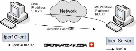
iPerf (https://iperf.fr) is a Layer 4 (TCP / UDP) emulator
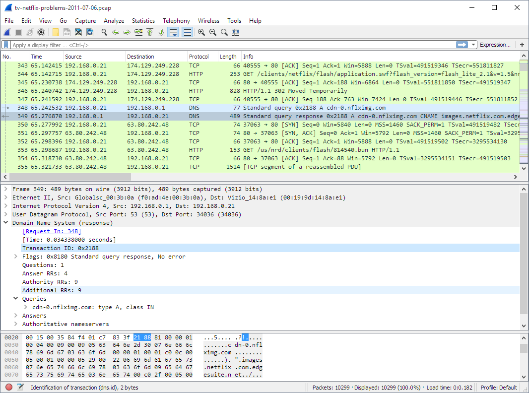
Wireshark (https://www.wireshark.org) is a Layer 4 (TCP / UDP) packet analyzer
iPerf
“iPerf3 is a tool for active measurements of the maximum achievable bandwidth on IP networks. It supports tuning of various parameters related to timing, buffers and protocols (TCP, UDP, SCTP with IPv4 and IPv6). For each test it reports the bandwidth, loss, and other parameters.”

Note: iPerf “bandwidth” corresponds to our notion of “throughput”.
WireShark
“Wireshark is a network packet analyzer. A network packet analyzer presents captured packet data in as much detail as possible…. Wireshark is available for free, is open source, and is one of the best packet analyzers available today.

