import numpy as np
import matplotlib.pyplot as pltLecture 06 - Digital Packets & Signaling
EE-30023/31023, Department of Electrical Engineering, University of Notre Dame
Summary
In this lecture, we summarize digital streams, packets formats, and signaling as they are widely used for both wireline and wireless transmissions.
Motivation in Course Context
Information sources are today represented in a variety of digital formats, i.e., representations consisting of sets of \(0\)’s and \(1\)’s.
In the next three lectures, we summarize concepts of digital data packets and network stacks that modern digital radios have to support.
Our outline will be as follows:
Digital Packets and Signaling (1/24)
Layered Protocols for Networking (1/26)
Link Performance Metrics (1/28)
Information in Digital Formats
Discussion: What information sources are now digital?
Text (ASCII, https://en.wikipedia.org/wiki/ASCII; Unicode, https://en.wikipedia.org/wiki/Unicode)
Speech (AMR, https://en.wikipedia.org/wiki/Adaptive_Multi-Rate_audio_codec)
Audio (MP3, https://en.wikipedia.org/wiki/MP3)
Images (JPEG, https://en.wikipedia.org/wiki/JPEG)
Video (MP4, https://en.wikipedia.org/wiki/MPEG-4_Part_14)
…
Is there any information today that is not represented as digital? Vynyl records, old photographs, AM & FM radio broadcasting.
Digital Representation Terminology
A binary digit, often abbreviated as a bit, is a value \(b\in\{0,1\}\).
A bit stream is an arbitrarily large sequences or string of bits, \(b[n],n\in\mathbb{Z}\).
A frame or a packet is a finite-length sequence or string of bits, \(b[n],n\in\{0,1,\ldots,N-1\}\).
A subframe or a field is a finite-length sequence of string of bits defined as a part of a frame.
Example: The MP4 standard defines a “transport stream” as a sequence of “transport frames”, and each transport frame may contain video and audio frames.
Wireline Communication Standards
Exploration: Standards documents are great places to see how communication engineers specify systems, and learning what we need to learn!
Each of these standards involves physical specifications for the wire media and connectors, electrical circuit interfaces to the media, signaling formats, and packet structures.
A brief summary of these signaling formats is shown in the table below.
TBD
General Packet Structure
Reviewing these communication standards (and many others), we see that there is a general format to digital frames or packets as illustrated in Figure 1.
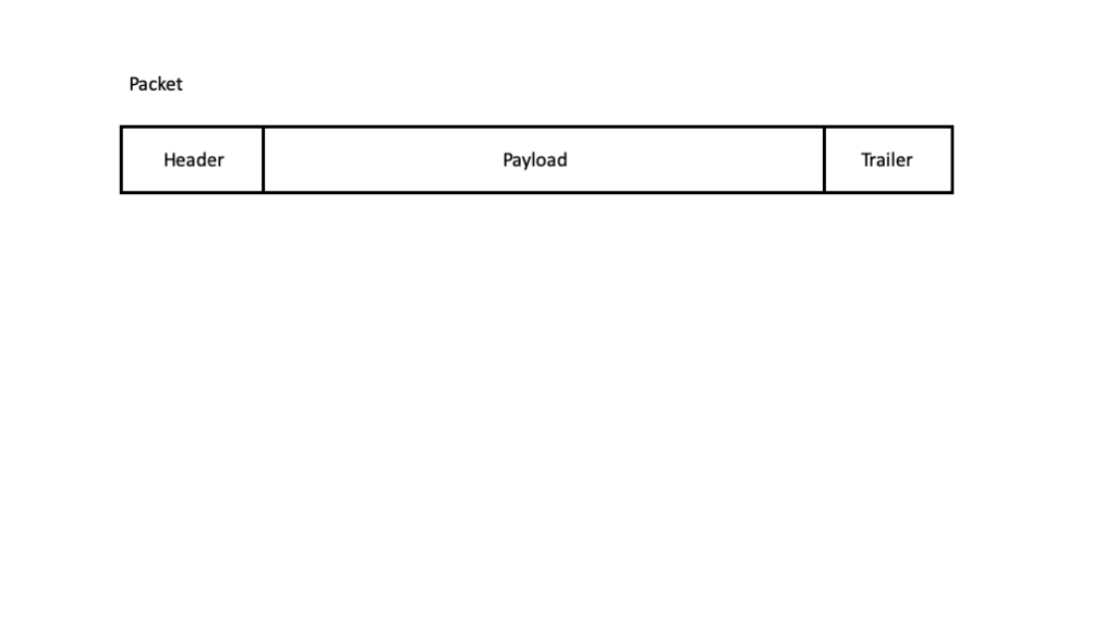
The three high-level fields of a packet include:
Header - Often includes subfields for synchronization, identifying the packet format, specifying the packet length, addressing, and so forth.
Payload - Contains the data as one or more sub-packets, can be variable length depending upon the protocol.
Trailer - When used, can include error detection and synchronization subfields.
Digital Signaling Waveforms
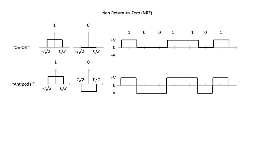
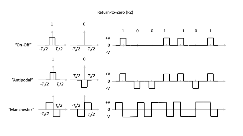
Mathematical Models
Now we can formulate mathematical models for these signaling formats. In our notation, let \(T\) denote the bit, or symbol, period, so that \(R=1/T\) denotes the data rate in bits per second.
The following are the mathematical relationships for various signaling formats.
NRZ: \[ \sum_{n} A_n\ \mathrm{rect}\left( \frac{t-nT}{T} \right) \tag{1}\]
RZ: \[ \sum_{n} A_n\ \mathrm{rect}\left( \frac{t-nT}{T_0} \right) \tag{2}\] where \(T_0 < T\)
Manchester: Let \[ p(t)=\mathrm{rect}\left( \frac{t+T/4}{T/2} \right) - \mathrm{rect}\left( \frac{t-T/4}{T/2} \right) \] then \[ \sum_{n} A_n\ p\left( \frac{t-nT}{T} \right) \tag{3}\]
To complete the signal formats, we have to specify the values taken by the \(\{A_n\}\):
On-Off Keying: \[ A_n = \begin{cases} +V & b[n] = 1 \\ 0 & b[n] = 0 \end{cases} \tag{4}\]
Antipodal: \[ A_n = \begin{cases} +V & b[n] = 1 \\ -V & b[n] = 0 \end{cases} \tag{5}\]
We see from these relationships that we can generate these digital signaling waveforms with the same signals and systems concepts as interpolation!
Bandwidth
Given the prevalence of rectangular pulse waveform in these digital signaling formats, a natural issue to consider is the “bandwidth” of the transmission.
Given the Fourier transform relationship \[ p(t)=\mathrm{rect}(t/T) \leftrightarrow P(f)=T\mathrm{sinc}(fT) \tag{6}\] for general \(T\), we know that this waveform and waveforms derived from it are not bandlimited in a strict sense.
We can compare the Fourier transforms of the various signaling formats as shown in the figures below. We start by importing our NumPy and Matplotlib libraries.
Next we define the symbol period \(T\), the multipler \(W\) of \(1/T\) we will use in the frequency domain, and the values of frequency \(f\) to plot.
T = 1e-6
W = 10.5
f = np.linspace(-W/T,W/T,4000)
NRZ Waveform
We begin with the NRZ waveform.
NRZ = T*np.sin(np.pi*f*T)/(np.pi*f*T)The plot below illustrates the magnitude response of this Fourier transform, where we have appropriately normalized the vertical axis by \(T\) and the horizonal axis by \(1/T\). We observe that the waveform is not bandlimited, but the magnitude response decays to \(0\) like \(1/f\) as \(f \rightarrow \infty\).
plt.plot(f*T,np.abs(NRZ/T),'-',label='NRZ')
plt.legend()
plt.xlabel('$fT$')
plt.ylabel('$|P(f)/T|$');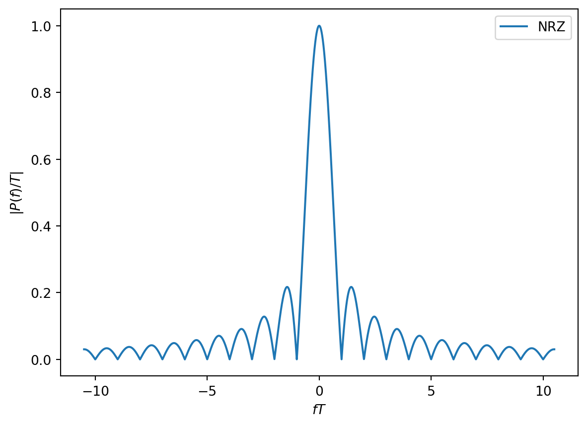
The magnitude response equals zero for \(f=k/T\), where \(k\in\mathbb{Z}-\{0\}\). We refer to the portion of the magnitude response for \(f\in[-1/T,+1/T]\) as the main lobe, and every other interval \(f\in[k/T,(k+1)/T)\) \(k=2,3,\ldots\) as successive side lobes.
We define the main lobe bandwidth as the smallest positive frequency such that \(|P(f)|=0\). In the case of the rectangular NRZ waveform with bit or symbol period \(T\), we see that the main lobe bandwidth is \(1/T\), which corresponds to the data rate \(R\). Thus, transmitting higher data rates requires larger signal bandwidth in the NRZ signaling format.
The plot below illustrates the magnitude response on a decibel (dB) scale and for narrower range of \(fT\).
plt.plot(f*T,20.0*np.log10(np.abs(NRZ/T)),'-',label='NRZ')
plt.axis([-5,5,-40,0])
plt.legend()
plt.xlabel('$fT$')
plt.ylabel('$|P(f)/T|$ (dB)');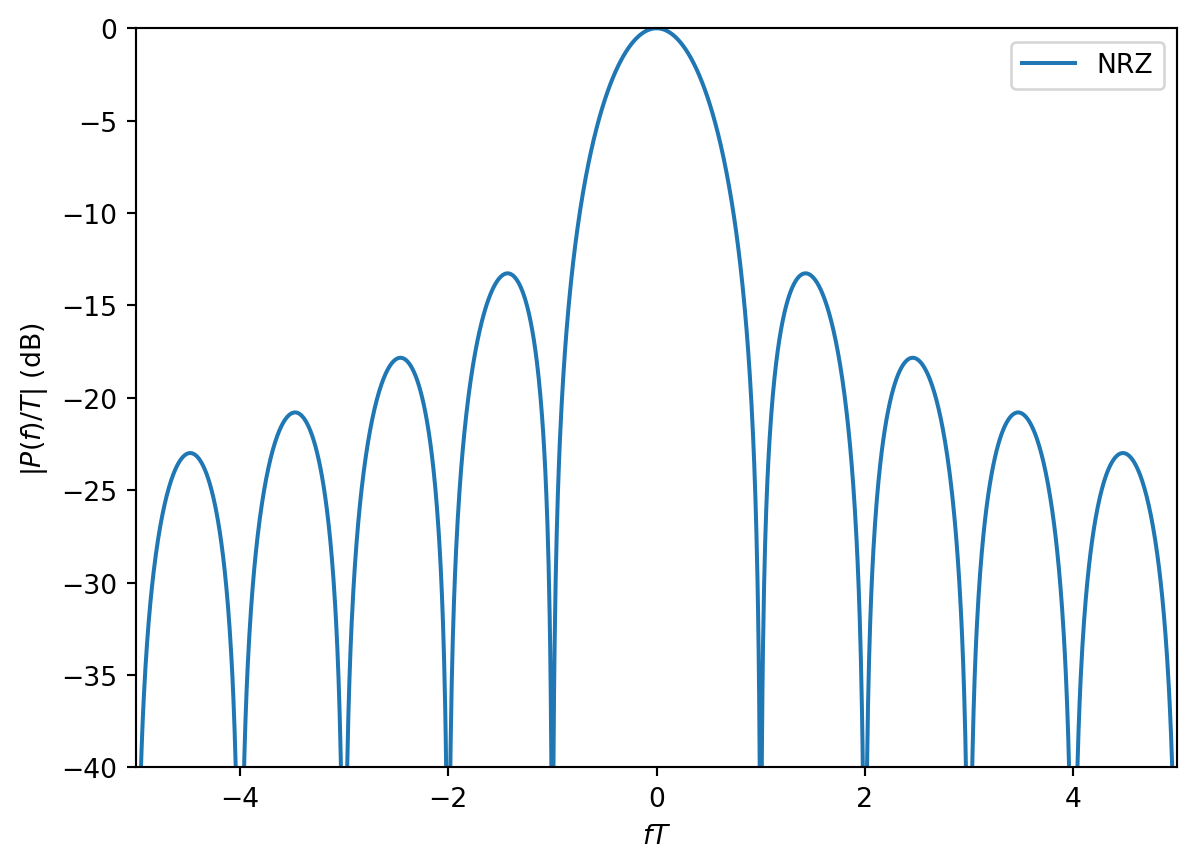
RZ Waveform
Now we consider a RZ waveform with 50% duty cycle, i.e., \(T_0 = T/2\).
T0 = 0.5*T
RZ = T0*np.sin(np.pi*f*T0)/(np.pi*f*T0)
In the plot of the magnitude response of this waveform, we see that it has twice the main lobe bandwidth. More generally, the main lobe bandwidth of the RZ waveform is \(1/T_0\). In this case, we observe that the main lobe bandwidth is actually larger than the data rate! However, as we grow the data rate by increasing \(R=1/T\), we still increase the banwidth since \(1/T_0 > 1/T\).
plt.plot(f*T,20.0*np.log10(np.abs(RZ/T)),'-',label='RZ');
plt.axis([-5,5,-40,0])
plt.legend()
plt.xlabel('$fT$')
plt.ylabel('$|P(f)/T|$ (dB)');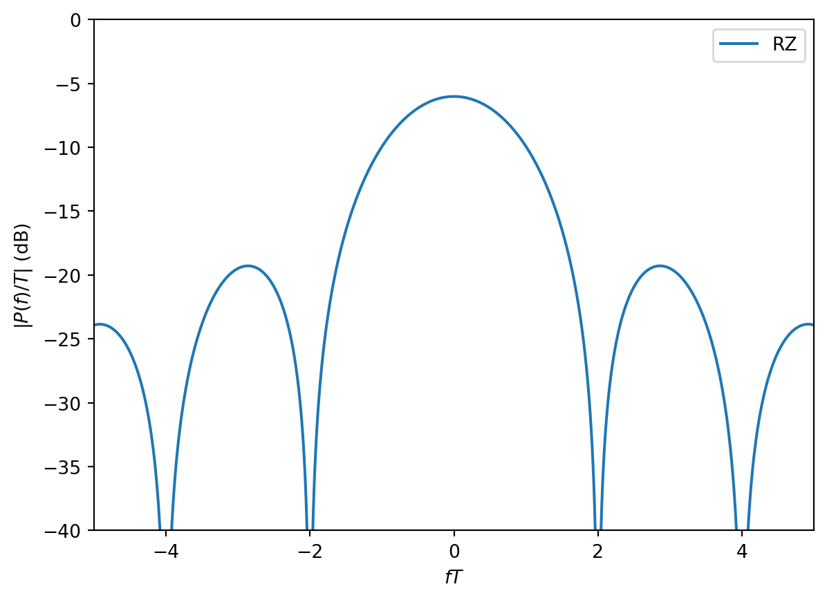
Manchester Waveform
The time-domain waveform \[ p(t)=\mathrm{rect}\left( \frac{t+T/4}{T/2} \right) - \mathrm{rect}\left( \frac{t-T/4}{T/2} \right) \] has Fourier transform \[ P(f) = e^{j2\pi f \frac{T}{4}} \frac{T}{2} \mathrm{sinc}\left( \frac{fT}{2} \right) - e^{-j2\pi f \frac{T}{4}} \frac{T}{2} \mathrm{sinc}\left( \frac{fT}{2} \right) = j T \sin\left( \frac{\pi f T}{2} \right) \mathrm{sinc}\left( \frac{fT}{2} \right) \] We should not be surprised that this Fourier transform is purely imaginary, because the time-domain waveform is odd symmetric.
MAN = 1j*T*np.sin(np.pi*f*T/2)*np.sin(np.pi*f*T/2)/(np.pi*f*T/2)plt.plot(f*T,np.imag(MAN/T),'-',label='MAN')
plt.legend()
plt.xlabel('$fT$')
plt.ylabel('$\mathrm{Im}\{P(f)/T\}$');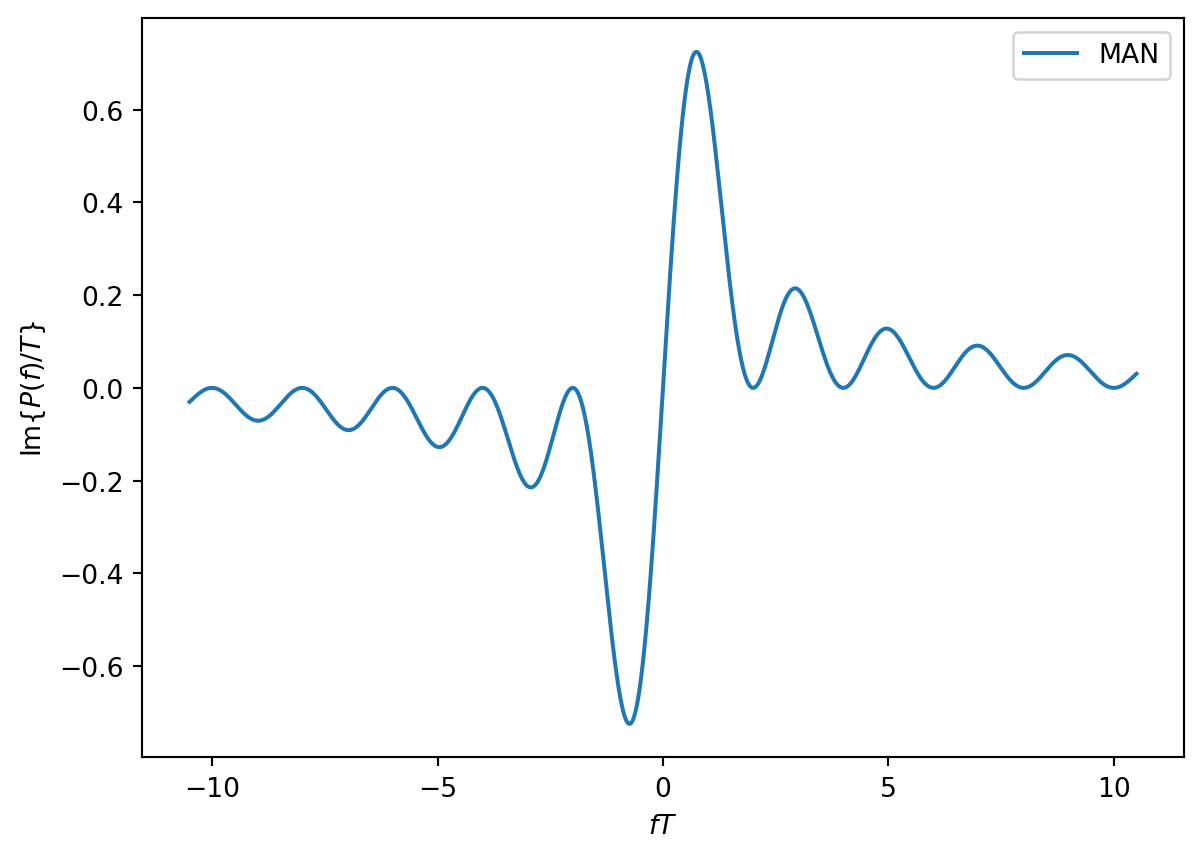
plt.plot(f*T,20.0*np.log10(np.abs(MAN/T)),'-',label='MAN');
plt.axis([-5,5,-40,0])
plt.legend()
plt.xlabel('$fT$')
plt.ylabel('$|P(f)/T|$ (dB)');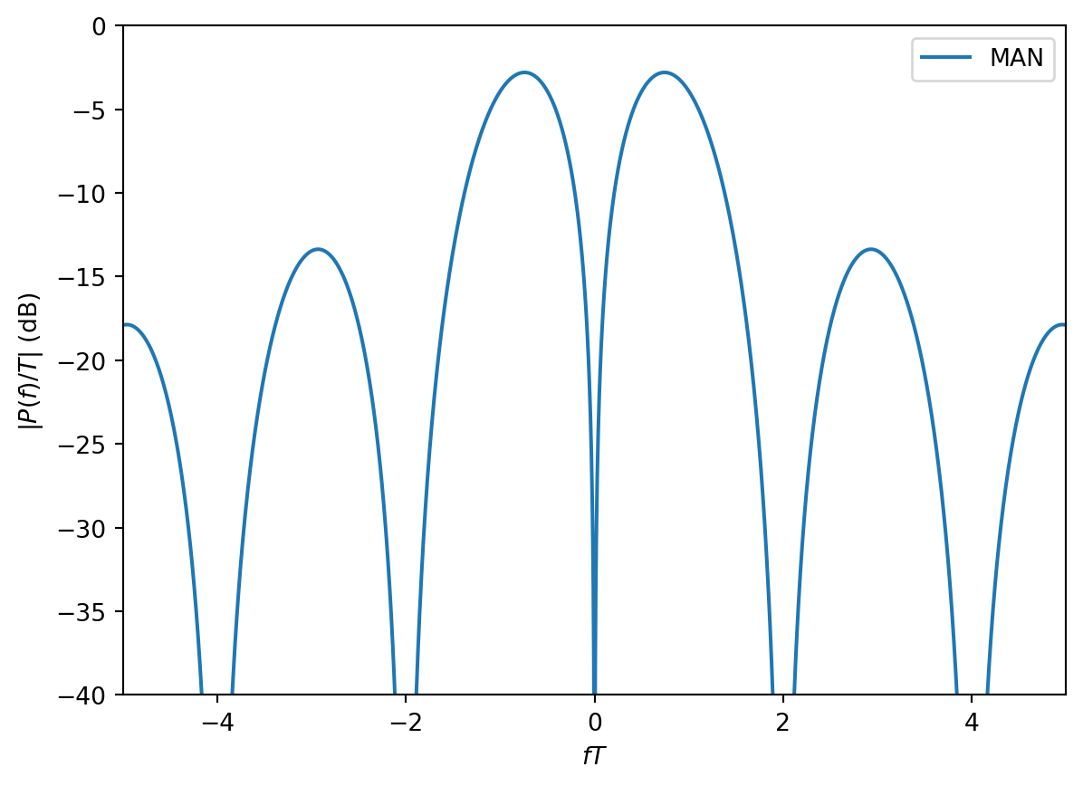
Not surprisingly, we see that the Manchester waveform has main lobe bandwidth \(2/T\) like the 50% duty cycle rectangular waveform from which it is formed. However, the Manchester waveform has no DC component in the frequency domain.
