Code
import numpy as np
import scipy.signal as sig
import matplotlib.pyplot as pltEE-30023/31023, Department of Electrical Engineering, University of Notre Dame
We can demonstrate the pulse shaping we’ve learned thus far in discrete time using Python.
We’ll begin by importing a few libraries that will make our lives much simpler.
import numpy as np
import scipy.signal as sig
import matplotlib.pyplot as pltNext, we generate a random stream of data. In a real communication system this data would come from something that was being sent, like an image or a webpage, but for now we will generate it randomly.
Our data will be in the form of QPSK symbols with energy per bit \(E_b = 1\). We can generate 100 symbols as follows:
N = 100
a_r = 2.0*np.random.randint(2, size=N)-1.0
a_i = 2.0*np.random.randint(2, size=N)-1.0
a = a_r + 1j*a_i
We can see these random signals in the figure below, where the blue points indicate the real part of the symbols and the red part indicates the imaginary part.

We can select an oversampling factor which equates to the number of samples per symbol. For our purposes, a larger number here will make the waveforms smoother so we choose 100.
M = 100We now create our first (and simplest) pulse shaping filter: a delta function. We will use this delta to upsample our input symbols.
p_delta = np.zeros(M)
p_delta[0] = 1
Next we create another simple filter: the rectangle filter. We know that this filter is not ideal in wireless situations because it is not bandlimited, but we will use it to demonstrate that effect.
p_rect = np.ones(M) / np.sqrt(M)
The next filter we will create is the raised cosine filter. We know that this filter satisfies the Nyquist criterion for zero ISI, so it is useful in wireless transmission.
def rcos(alpha, L=5, T=1.0):
    Ts = T/M
    t = np.arange(2*L*M+1)*Ts-L*T

    if alpha == 0:
        return np.sinc(t/T)

    h = np.zeros(np.size(t))
    for i in range(np.size(h)):
        if t[i]==T/(2*alpha) or t[i]==-T/(2*alpha):
            h[i] = np.pi*np.sinc(1/(2*alpha)) / 4 / T
        else:
            h[i] = np.sinc(t[i]/T) * np.cos(np.pi * alpha * t[i] / T) / (1-(2*alpha*t[i] / T)**2)
    return h

alpha = 0.25    # excess bandwidth
p_rc = rcos(alpha)
p_rc = p_rc / np.sqrt(np.sum(p_rc**2)) # normalize for unit energy
The final filter we’ll create is the root-raised cosine filter. As we’ve discussed, using a root-raised cosine filter at both the transmitter and the receiver gives us the properties of a single raised cosine while allowing for optimal detection using a matched filter.
def rrcos(alpha, L=5, T=1.0):
    Ts = T/M
    t = np.arange(2*L*M+1)*Ts-L*T

    if (alpha==0.0):
        return np.sinc(t/T) / np.sqrt(T)

    h = np.zeros(np.size(t))
    for i in range(np.size(h)):
        if t[i] == 0.0: # See MR Problem A.6
            h[i]= (1/np.sqrt(T)) * (1- alpha + 4*alpha / np.pi)
        else:
            if t[i]==T/(4*alpha) or t[i]==-T/(4*alpha): # See MR Problem A.6
                h[i] = (alpha/np.sqrt(2*T)) * ((1+2/np.pi)*np.sin(np.pi/4/alpha) + (1-2/np.pi)*np.cos(np.pi/4/alpha))
            else: # MR Equation A.30
                h[i] = (1/np.sqrt(T)) * (np.sin(np.pi*(1-alpha)*t[i]/T) + (4*alpha*t[i]/T) * np.cos(np.pi*(1+alpha)*t[i]/T)) / (1-(4*alpha*t[i]/T)**2) / (np.pi*t[i]/T)
    return h

alpha = 0.25    # excess bandwidth
p_rrc = rrcos(alpha)
p_rrc = p_rrc / np.sqrt(np.sum(p_rrc**2)) # normalize for unit energy
We can apply the upsampling filter using a function from Scipy called upfirdn. The function first upsamples the signal a by a factor M, then applies the filter p_delta, then downsamples by another factor. We choose here to not specify a downsampling factor, so no downsampling occurs. We can see that the x-axis now goes all the way to 10000 instead of 100 because there are 100 samples per symbol now.
u = sig.upfirdn(p_delta, a, M)
We can use upfirdn again to actually apply our pulse shaping filter. First, let’s select a rectangle filter and see what our pulse-shaped signal looks like:
s = sig.upfirdn(p_rect, a, M)
The frequency domain view of the signal shows us why the rectangle filter is not ideal for wireless communication:
S = np.fft.fft(s)
S = np.fft.fftshift(S) / len(S)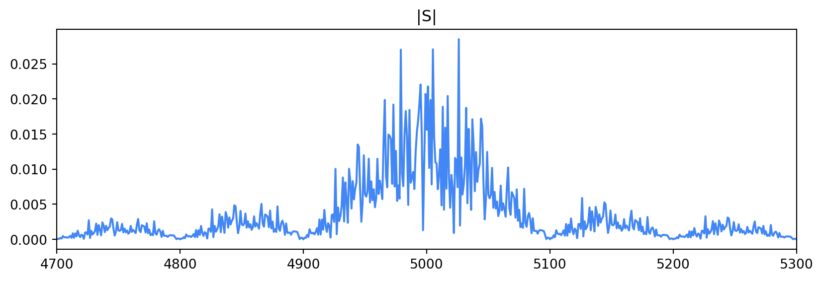
We see that the magnitude of the fourier transform of our signal has an infinite bandwidth. In bandlimited situations, this is unacceptable. Let’s use the root-raised cosine filter and see how this picture changes.
s = sig.upfirdn(p_rrc, a, M)
It has the corresponding frequency spectrum
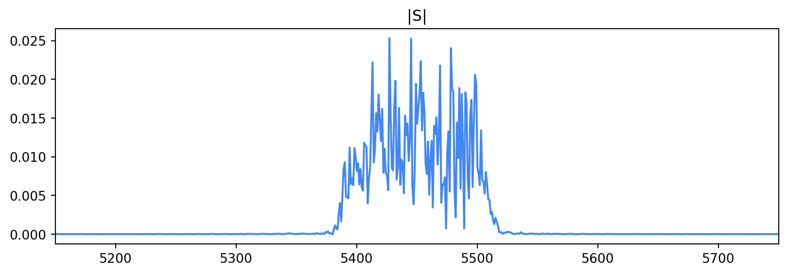
We can see that the signal is bandlimited, exactly as we want. Changing the value of the excess bandwidth will affect how much bandwidth we require. A smaller excess bandwidth is good in the frequency domain because it allows us to push more data through a channel with less bandwidth. There are consequences for a low excess bandwidth in the time domain, however.
We can use a diagram called an Eye Diagram to take a closer look at the transition between symbols in our signal. With this view, we can better evaluate if there is any ISI in our signal. Let’s first look at the root-raised cosine eye diagram on the transmit side:
p_rrc = rrcos(0.25)
s = sig.upfirdn(p_rrc, a, M)

delay = int((len(p_rrc)-1)/2) # truncate the first and last few symbols
window = 2*M                   # show 2 symbols periods
for k in range(int((len(s)-2*delay) / window)):
    plt.plot(np.real(s)[delay + (k*window):delay + ((k+1)*window)], blue)
    plt.plot(np.imag(s)[delay + (k*window):delay + ((k+1)*window)], red)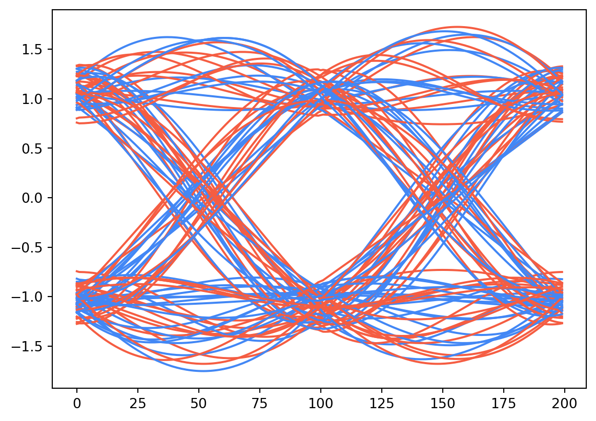
Keep in mind, though, that this is our transmitted waveform. We still need a matched filter on the receiver before we can do minimum distance detection. If we apply the matched filter, the story changes:
r = sig.upfirdn(p_rrc, s)

delay = int((len(p_rrc)-1)) # truncate the first and last few symbols
window = 2*M                # show 2 symbols periods
for k in range(int((len(r)-2*delay) / window)):
    plt.plot(np.real(r)[delay + (k*window):delay + ((k+1)*window)], blue)
    plt.plot(np.imag(r)[delay + (k*window):delay + ((k+1)*window)], red)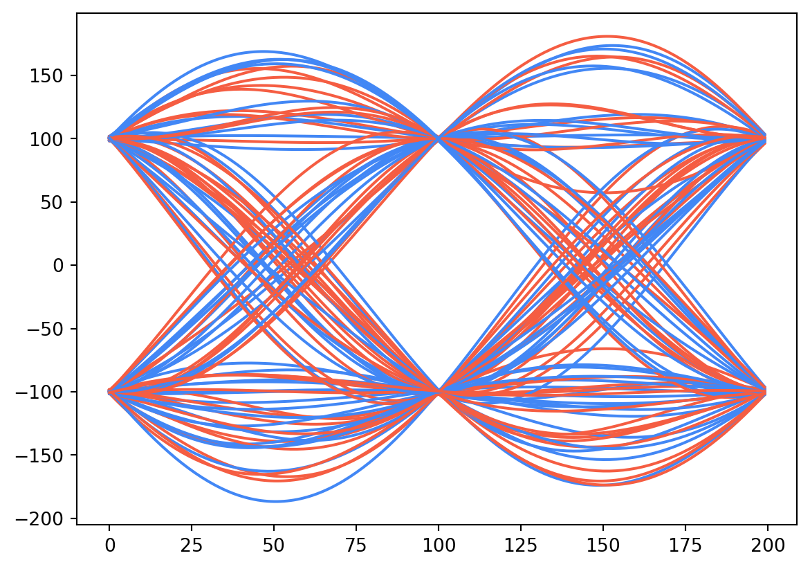
We can see that the root-raised cosine pulse with a moderate amount of excess bandwidth can completely eliminate ISI. For demonstration purposes, we can show what the eye diagram would like like for a filter with different values of excess bandwidth:
plt.figure(figsize=(11, 12))
for i, alpha in enumerate([0, .01, .05, .1, .25, .5]):
    p_rrc = rrcos(alpha)
    s = sig.upfirdn(p_rrc, a, M)
    r = sig.upfirdn(p_rrc, s)

    delay = int((len(p_rrc)-1)) # truncate the first and last few symbols
    window = 2*M                # show 2 symbols periods
    plt.subplot(3, 2, i+1)
    plt.title(rf"$\alpha={alpha}$")

    for k in range(int((len(r)-2*delay) / window)):
        plt.plot(np.real(r)[delay + (k*window):delay + ((k+1)*window)], blue)
        plt.plot(np.imag(r)[delay + (k*window):delay + ((k+1)*window)], red)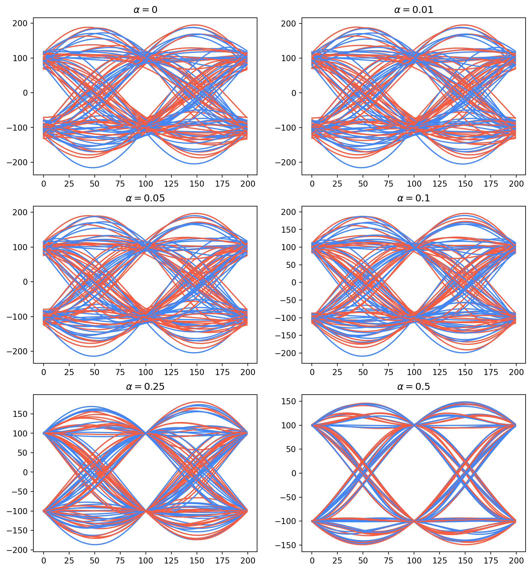
We see (as expected) that using more bandwidth leads to cleaner transitions between symbols and thus makes it easier to minimum distance detection.