Lecture 02 - Signals, Systems, and Transforms

Summary

In this lecture, we will review some of the important concepts and terminology, and our notation, from what is commonly called signals and systems.

We focus initially on single-input, single-output, linear time-invariant (LTI) systems. The key idea in LTI systems is that their effect on complex exponential signals is particularly simple. This motivates transforms between the time domain and frequency domain through we represent general signals as linear combinations of complex exponentials.

We address these notions in both continuous-time domain and discrete-time domain, and set the stage for connecting the two domains in the next lecture.

Motivation in Course Context

Three important components for modeling the radio system architectures that we discussed in the previous lecture are 1) an digital-to-analog converter (DAC) in the transmitter, 2) a propagation “channel” that we aim to model as a linear, time-varying filter, and 3) the analog-to-digital converter (ADC) in the receiver. A block diagram for such a system model is shown in Figure 1.

Figure 1: Radio transmission system model

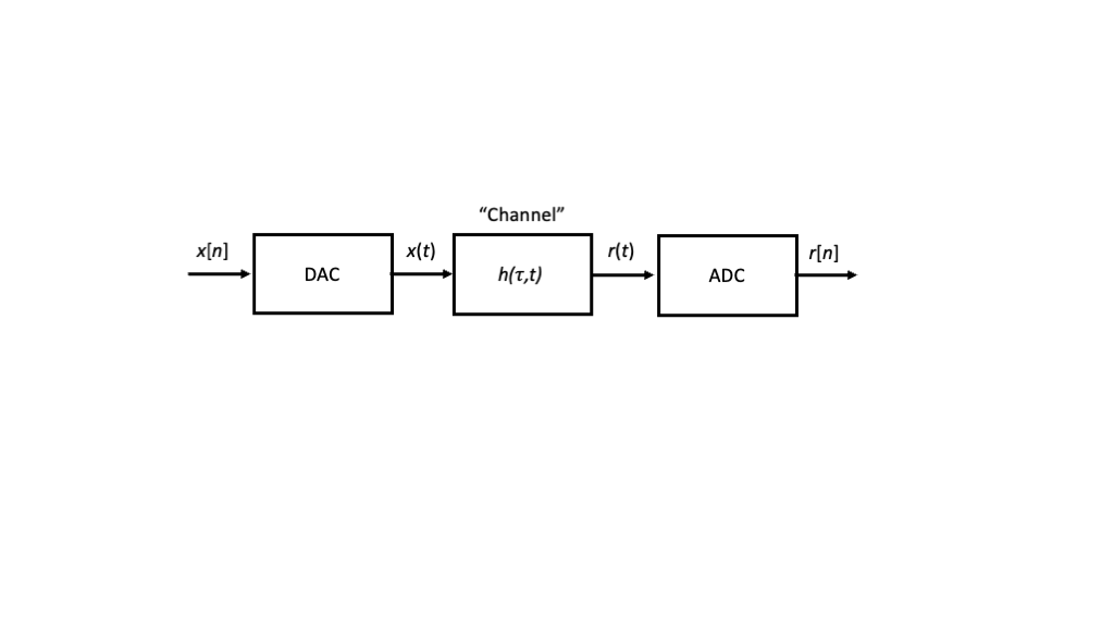
In this lecture, we review the background material required to treat these inputs and outputs as continuous-time signals and discrete-time sequences, and we develop the appropriate notions of the frequency domain and the important class of linear time-invariant (LTI) systems. In our next lecture, we will address sampling, interpolation, and quantization aspects of DACs and ADCs.

Signals and Sequences

When we wire up an electrical circuit, we can use an instrument to measure a voltage or current, either of which typically varies over time.

Mathematically, we denote time by the real variable $t\in \mathbb{R}$, which we refer to as the continunous-time axis, and we denote the voltage or current by the real-valued functions $v(t)$ and $i(t)$, respectively.

More generally, we can consider any quantity that varies as a function of time as a signal, and we generically denote it by $s(t)$. As other examples, we could measure the temperature in a room, or the price of a stock, or … as functions time.

If, for whatever reason, we are only able to measure a signal at the discrete time instants $t=n{T}_s$ for integer $n\in \mathbb{Z}$, which we refer to as the discrete-time axis, we denote the sequence by $s[n]=s(n{T}_s)$, accordingly. Although the time axis is discrete in the variable $n$, in general $s[n]$ can take real values.

In this context, we refer to the value $x[n_0]$ as the sample of $x(t)$ for $t=n_0{T}_s$, $n_0\in \mathbb{Z}$. We refer to the spacing between samples in time $T_s$ as the sampling period, and we define $f_s=1/T_s$ as the sampling frequency.

Finally, we often consider complex-valued signals and sequences such as $$s(t)=s_R(t)+j{s}_I(t)$$ $$s[n]=s_R[n]+j{s}_I[n]$$ where $s_R(t)$ and $s_I(t)$ are real-valued signals, $s_R[n]$ and $s_I[n]$ are real-valued sequences, and $j=\sqrt{-1}$ is the standard notation for the unit imaginary number in the field of electrical engineering.

Simple Signals

In this section, we define and visualize a number of simple signals.

Constant Signal

The simplest possible signal is the constant signal for which $s(t)=A$ for some constant value $A\in \mathbb{R}$ and all $t\in \mathbb{R}$.

That is, the constant signal takes the same value for all time.

Rising Exponential Signal

Another simple signal is the rising exponential signal $$\begin{array}{}\text{(1)}& r_{\tau }(t):=\{\begin{array}{ll}1-e^{-t/\tau }& t\ge 0\\ 0& t<0\end{array},\end{array}$$ where $\tau >0$ is called the time constant.

Since $e^{-t/\tau }$ decays to $0$ as $t$ becomes large, i.e., $\underset{t\to \mathrm{\infty }}{lim}{e}^{-t/\tau }=0$, we see that $r_{\tau }(t)$ approaches $1$ as $t$ becomes large, i.e., $\underset{t\to \mathrm{\infty }}{lim}{r}_{\tau }(t)=1$.

How fast $r_{\tau }(t)$ approaches $1$ depends upon the time constant $\tau$: larger values of $\tau$ cause $r_{\tau }(t)$ to approach $1$ more slowly, and smaller values of $\tau$ cause $r_{\tau }(t)$ to approach $1$ more rapidly.

This is illustrated in the simple numerical calculation and plot below.

import numpy as np
import matplotlib.pylab as plt

tau1 = 1
tau2 = 4
t=np.linspace(0,20,40)
r1 = 1-np.exp(-t/tau1)
r2 = 1-np.exp(-t/tau2)

label1 = "$\\tau="+str(tau1)+"$"
label2 = "$\\tau="+str(tau2)+"$"
plt.plot(t,r1,'s-',label=label1)
plt.plot(t,r2,'s-',label=label2)
plt.xlabel('$t$')
plt.ylabel('$r_{\\tau}(t)$')
plt.legend()
plt.show()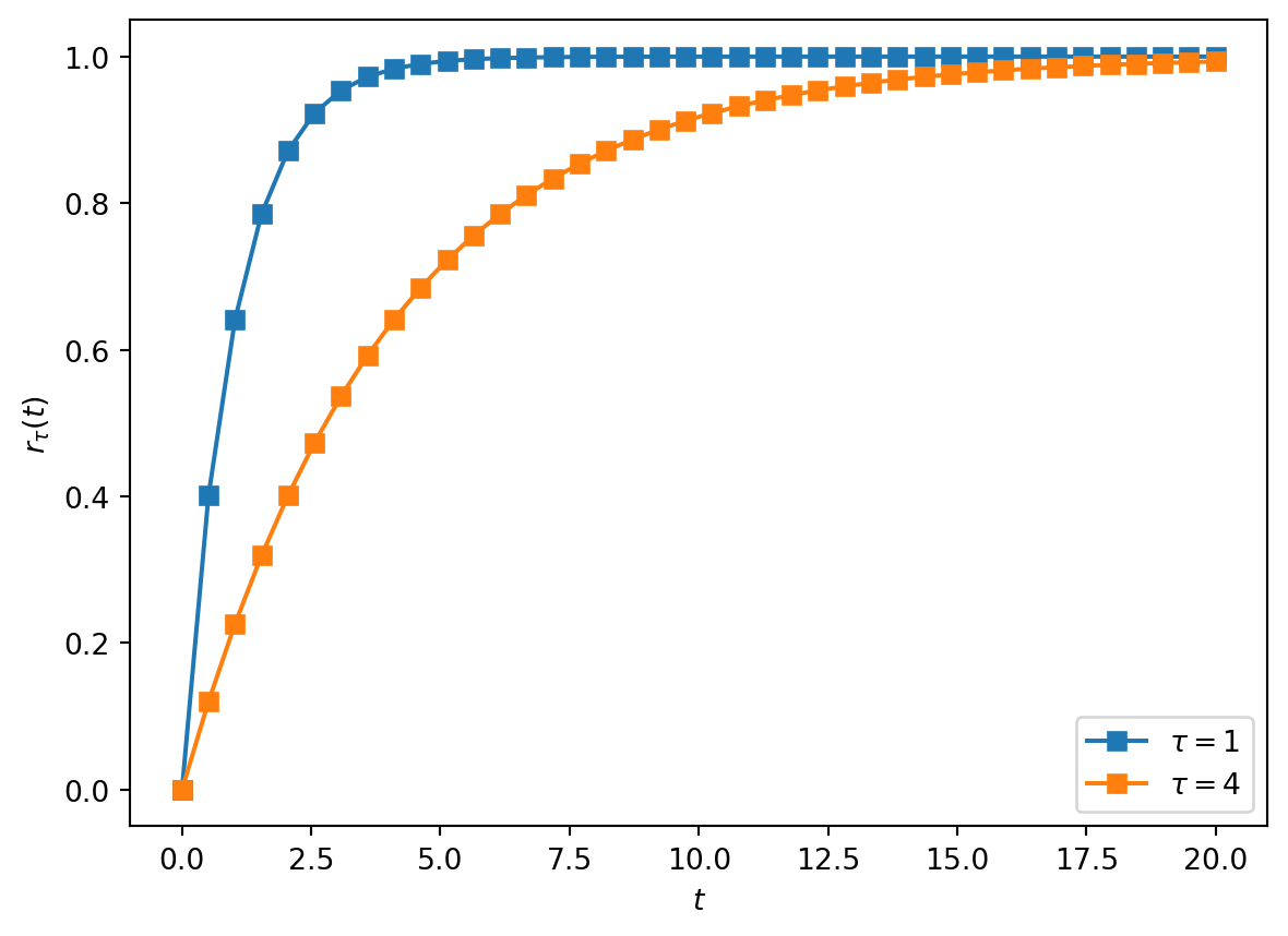

EXERCISE: Verify that, to achieve $r_{\tau }(t)\ge 0.99$, we require $t\ge -\ln (0.01)\cdot \tau \approx 4.6\cdot \tau$.

Thus, a good rule of thumb is that a rising exponential signal essentially converges to its limit after five time constants. The duration $5\tau$ is sometimes called the rise time of the rising exponential signal.

Unit Step Signal

Another simple signal is the unit step signal $$\begin{array}{}\text{(2)}& u(t):=\{\begin{array}{ll}1& t>0\\ 0& t\le 0\end{array}.\end{array}$$ That is, the unit step signal “turns on” after time $t=0$ after being “off” for $t\le 0$.

Notice that the unit step can be viewed as a pointwise limit of the rising exponential signal as $\tau$ approaches $0$, i.e., $u(t)=\underset{\tau \to 0}{lim}{r}_{\tau }(t)$ for all $t\in \mathbb{R}$.

On one hand, the mathematical expression for $u(t)$ is simpler than that of the rising exponential signal, so $u(t)$ can be a convenient approximation to the rising exponential signal for small $\tau$.

On the other hand, $u(t)$ is discontinuous at $t=0$, whereas the rising exponential signal is continuous for all $t$.

EXERCISE: Verify that $$u(t-\tau )=\{\begin{array}{ll}1& t>\tau \\ 0& t\le \tau \end{array}.$$ In words, the delayed unit step signal $u(t-\tau )$ is off for $t\le \tau$ and on for $t>\tau$.

Rectangular Signal

Another simple signal is the rectangular signal $$\begin{array}{}\text{(3)}& \mathrm{rect}(t):=u(t+\frac{1}{2})-u(t-\frac{1}{2}).\end{array}$$

EXERCISE: Verify that $$\mathrm{rect}(t)=\{\begin{array}{ll}1& |t|<\frac{1}{2}\\ 0& |t|\ge \frac{1}{2}\end{array}.$$ In words, the rectangular signal $\mathrm{rect}(t)$ is off for $t\le -1/2$, turns on for $-1/2<t<+1/2$, and then turns off for $t>+1/2$.

EXERCISE: Determine a simple expression for $\mathrm{rect}(t/T)$ for $T>0$.

Dirac Delta Signal

Another signal that is actually defined in terms of a pointwise limit of functions is the Dirac delta signal $$\begin{array}{}\text{(4)}& \delta (t):=\underset{ϵ\to 0}{lim}{\delta }_{ϵ}(t),t\in \mathbb{R},\end{array}$$ where ${\delta }_{ϵ}(t)$ is a set of functions parameterized by $ϵ>0$ satisfying $$\begin{array}{}\text{(5)}& {\int }_{-\mathrm{\infty }}^{+\mathrm{\infty }}{\delta }_{ϵ}(t)dt=1,ϵ>0,\end{array}$$ and $$\begin{array}{}\text{(6)}& \underset{ϵ\to 0}{lim}{\delta }_{ϵ}(t)=\{\begin{array}{ll}+\mathrm{\infty }& t=0\\ 0& t\ne 0\end{array}.\end{array}$$

The simplest such set of functions is given by $${\delta }_{ϵ}(t)=\frac{1}{ϵ}\mathrm{rect}\left(\frac{t}{ϵ}\right)=\{\begin{array}{ll}\frac{1}{ϵ}& |t|<\frac{ϵ}{2}\\ 0& |t|\ge \frac{ϵ}{2}\end{array}.$$ That is, the ${\delta }_{ϵ}(t)$ functions are rectangular with width $ϵ$ and height $\frac{1}{ϵ}$, so that they become narrower and taller as $ϵ$ becomes smaller.

An important property satisfied by the Dirac delta signal is the sifting property, which states that for a signal $s(t)$, $t\in \mathbb{R}$, and for any $\tau \in \mathbb{R}$, $$\begin{array}{}\text{(7)}& {\int }_{-\mathrm{\infty }}^{+\mathrm{\infty }}s(t)\delta (t-\tau )dt=s(\tau ).\end{array}$$ In words, a Diract delta signal delayed by $\tau$ “sifts” out the value of the signal $s(t)$ for $t=\tau$ under the integral.

Sinusoidal Signals

Another very important class of signals are sinusoidal signals, such as $\cos (2\pi f_{0}t)$ and $\sin (2\pi f_{0}t)$ for all $t\in \mathbb{R}$ and a given $f_0>0$. If we define $T_0=1/f_0$, we observe the following interesting property: $$\cos (2\pi f_0(t+k{T}_0))=\cos (2\pi f_{0}t+k2\pi )=\cos (2\pi f_{0}t),k\in \mathbb{Z}.$$

In words, the sinusoidal signal $\cos (2\pi f_{0}t)$ is periodic with fundamental period $T_0=1/f_0$.

The parameter $f_0$ is called the frequency of the sinusoid, and represents the number of periods or cycles of the sinusoid in one second. The units of frequency are Hertz.

f_0 = 10
T_0 = 1/f_0
t = np.linspace(-2*T_0,2*T_0,4*20)
c = np.cos(2*np.pi*f_0*t)
s = np.sin(2*np.pi*f_0*t)

plt.plot(t,c,'s-',label='cos')
plt.plot(t,s,'s-',label='sin')
plt.xlabel('t')
plt.legend()
plt.show()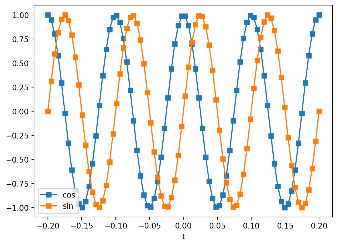

EXERCISE: Show that $\cos (2\pi f_{0}t+\pi /2)=\sin (2\pi f_{0}t)$, i.e., the $\cos$ “leads” the $\sin$, or the $\sin$ “lags” the $\cos$, by $\pi /2$ radians or ${90}^{\circ }$.

Continuous-Time Complex Exponential Signals

The last class of simple signals we will mention are complex exponential signals of the form $e^{j2\pi f_{0}t}$ for all $t\in \mathbb{R}$ and a given $f_0\in \mathbb{R}$, where $j=\sqrt{-1}$.

Using Euler’s relation, we have $$\begin{array}{}\text{(8)}& e^{j2\pi f_{0}t}=\cos (2\pi f_{0}t)+j\sin (2\pi f_{0}t).\end{array}$$ That is, the complex exponential signal has the $\cos$ and $\sin$ signals of a given frequency as its real and imaginary parts, respectively.

The following plot shows the $\cos$ and $\sin$ signals from the previous example in the complex plane (XY mode). The complex exponential cycles around the unit circle $f_0$ times per second. Specifically, for this example with $f_0>0$ and comparing to the previous figure, the complex exponential starts at the point $(1,0)$ and rotates counter clockwise through the points $(0,1)$, $(-1,0)$, and $(0,-1)$. For $f_0<0$, the complex exponential cycles clockwise around the unit circle $-f_0$ times per second.

plt.plot(c,s,'s-')
plt.xlabel('Real Part')
plt.ylabel('Image Part')
plt.show()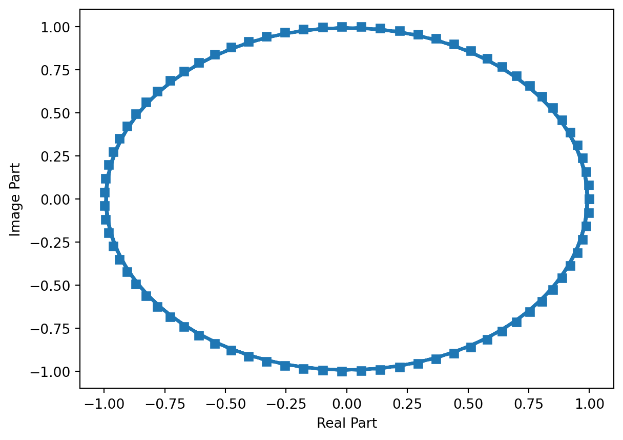

EXERCISE: Verify using Euler’s relation that $$\begin{array}{}\text{(9)}& \cos (2\pi f_{0}t)=\frac{1}{2}[e^{j2\pi f_{0}t}+e^{-j2\pi f_{0}t}]\end{array}$$ and $$\begin{array}{}\text{(10)}& \sin (2\pi f_{0}t)=\frac{1}{2j}[e^{j2\pi f_{0}t}-e^{-j2\pi f_{0}t}].\end{array}$$

EXERCISE: Verify using Euler’s relation the following trigonometric identities $$\begin{array}{}\text{(11)}& \cos (2\pi f_{1}t)\cos (2\pi f_{2}t)=\frac{1}{2}[\cos (2\pi (f_1-f_2)t)+\cos (2\pi (f_1+f_2)t)]\end{array}$$ $$\begin{array}{}\text{(12)}& \sin (2\pi f_{1}t)\sin (2\pi f_{2}t)=\frac{1}{2}[\cos (2\pi (f_1-f_2)t)-\cos (2\pi (f_1+f_2)t)]\end{array}$$ $$\begin{array}{}\text{(13)}& \cos (2\pi f_{1}t)\sin (2\pi f_{2}t)=\frac{1}{2}[\sin (2\pi (f_1+f_2)t)-\sin (2\pi (f_1-f_2)t)]\end{array}$$

Discrete-Time Complex Exponential Sequences

We can think of a discrete-time complex exponential sequence as samples of a continuous-time complex exponential signal, but some subtleties arise.

Consider $x(t)=e^{j2\pi ft}$ for a specific frequency $f\in \mathbb{R}$. Let $x[n]$ denote samples of this signal with sampling period $T_s$ (sampling frequency $f_s$), i.e., $x[n]=x(n{T}_s)$.

Then $$x[n]={e^{j2\pi ft}|}_{t=n{T}_s}=e^{j2\pi (f/f_s)n}$$ The ratio $f/f_s$ is called the normalized frequency of the discrete-time complex exponential, with units of cycles per sample.

If $f_s/f$ is an integer, the DT complex exponential is periodic, i.e., $x[n+k{N}_0]=x[n]$ for all $n\in \mathbb{Z}$. In this case, the period $N_0=f_s/f$, the inverse of the normalized frequency.

Now consider $y_k(t)=e^{j2\pi (f+k{f}_s)t}$, for a specific frequency $f\in \mathbb{R}$ and a specific integer $k\in \mathbb{Z}$. In words, the frequency of $y_k(t)$ is the frequency of $x(t)$ plus an integer multiple $k$ of the sampling frequency $f_s$.

The corresponding discrete-time complex exponential is $$y_k[n]={y_k(t)|}_{t=n{T}_s}=e^{j2\pi ((f+k{f}_s)/f_s)n}=e^{j2\pi k}{e}^{j2\pi (f/f_s)n}=e^{j2\pi (f/f_s)n}=x[n]$$ since $e^{j2\pi k}=1$, $k\in \mathbb{Z}$.

In words, the discrete-time samples corresponding to all continuous-time frequencies $f+k{f}_s$ are exactly the same. The continuous-time frequency $f+k{f}_s$ is said to alias to the frequency $f$, or the normalize frequency $f/f_s$, for all $k\in \mathbb{Z}$.

Another way to view this effect is that, for discrete-time sequences, the normalized frequency axis $(f/f_s)$ is periodic with fundamental period $1$.

We therefore focus on discrete-time normalized frequencies on the interval $[-1/2,+1/2]$ as a convention, and we use the variable $u$ to denote normalized frequencies.

Signal Energy and Power

We will often deal with finite-energy or finite-power signals.

The energy of a signal $s(t)$ is defined as $$\begin{array}{}\text{(14)}& E_s=\underset{T\to \mathrm{\infty }}{lim}{\int }_{-T/2}^{+T/2}|s(t){|}^{2}dt\end{array}$$ when the limit exists. The absolute value of the integrand is important for dealing with complex-valued signals.

The (average) power of a signal $s(t)$ is defined as $$\begin{array}{}\text{(15)}& P_s=\underset{T\to \mathrm{\infty }}{lim}\frac{1}{T}{\int }_{-T/2}^{+T/2}|s(t){|}^{2}dt\end{array}$$ when the limit exists.

EXERCISE: Verify that the energy and average power of the rectangular signal $\mathrm{rect}(t/T)$ are $E=T$ and $P=0$, respectively.

EXERCISE: Verify that the energy and average power of the complex exponential signal $e^{j2\pi f_{0}t}$ are $\mathrm{\infty }$ and $1$, respectively.

Similarly, the energy and (average) power of a sequence $s[n]$ are defined as $$\begin{array}{}\text{(16)}& E_s=\underset{N\to \mathrm{\infty }}{lim}\sum _{-N}^{+N}|s[n]{|}^2\end{array}$$ and $$\begin{array}{}\text{(17)}& P_s=\underset{N\to \mathrm{\infty }}{lim}\frac{1}{2N+1}\sum _{-N}^{+N}|s[n]{|}^2\end{array}$$ when the limits exist, respectively.

Correlation

For two signals $x(t)$ and $y(t)$, we define the correlation as $$\begin{array}{}\text{(18)}& <x(t),y(t)>:={\int }_{-\mathrm{\infty }}^{+\mathrm{\infty }}x(t)y^{\ast }(t)dt\end{array}$$

For two sequences $x[n]$ and $y[n]$, we define the correlation as $$\begin{array}{}\text{(19)}& <x[n],y[n]>:=\sum _{-\mathrm{\infty }}^{+\mathrm{\infty }}x[n]y^{\ast }[n]\end{array}$$

Two signals (sequences) are said to be orthogonal if there correlation is zero.

EXERCISE: Determine the correlation of $\mathrm{rect}(t/T)$ and $\mathrm{rect}((t-\tau )/T)$, $t\in \mathbb{R}$, for all values of $\tau ,T\in \mathbb{R}$. For which values of $\tau$, if any, are the two signals orthogonal?

EXERCISE: Determine the correlation of the signals $e^{j2\pi f_{1}t}$ and $e^{j2\pi f_{2}t}$, $t\in \mathbb{R}$, for all values of $f_1,f_2\in \mathbb{R}$. For which values of $f_1,f_2$, if any, are the signals orthogonal?

EXERCISE: Determine the correlaton of the sequences $e^{j2\pi u_{1}n}$ and $e^{j2\pi u_{2}n}$, $n\in \mathbb{Z}$, for all values of $u_1,u_2\in [-1/2,1/2]$. For which values of $u_1,u_2$, if any, are the sequences orthongonal?

Note: Be careful with aliasing effects!

Systems

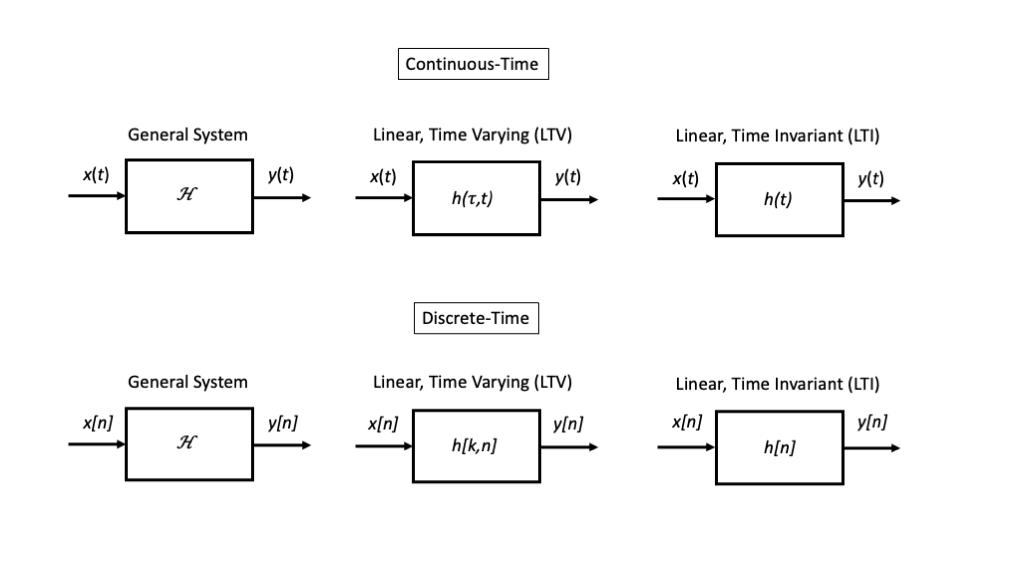
A system models the processing of input signal(s) or sequence(s) into output signal(s) or sequence(s). For starters, we will explore systems with a single input and a single output. Systems that process continuous-time signals are called continuous-time systems, and systems that process discrete-time sequences are called discrete-time systems.

For simplicity at this point, we denote a system by $\mathcal{H}$ and its response to input $x(t)$ by $\mathcal{H}\{x(t)\}$, and we draw such systems as components in block diagrams and shown in Figure 2.

Figure 2: System block diagrams in continuous-time and discrete-time

Simple Systems

Memoryless Operation

TBD

Delay / Advance

TBD

Time Limiter

TBD

Linear Time-Invariant Systems

Linearity and time-invariance are two very useful system properties that are satisfied by many systems. Systems that satisfy both properties are called linear, time-invariant (LTI) systems.

Definitions

A system $\mathcal{H}$ is linear if it satisfies two properties:

1. Scaling: If $y(t)=\mathcal{H}\{x(t)\}$, then input $\mathcal{H}\{ax(t)\}=ay(t)$ for all inputs $x(t)$ and all constaints $a\in \mathbb{C}$.
2. Superposition: If $y_1(t)=\mathcal{H}\{x_1(t)\}$ and $y_2(t)=\mathcal{H}\{x_2(t)\}$, then $\mathcal{H}\{a{x}_1(t)+b{x}_2(t)\}=a{y}_1(t)+b{y}_2(t)$, for all inputs $x_1(t)$ and $x_2(t)$ and all constants $a,b\in \mathbb{C}$.

A system is time-invariant if, for $y(t)=\mathcal{H}\{x(t)\}$, $\mathcal{H}\{x(t-\tau )\}=y(t-\tau )$ for all inputs $x(t)$ and all constants $\tau \in \mathbb{R}$.

In other words, delaying an input produces the same delay in the corresponding output.

Convolution Defines the LTI Input-Output Relationship

The input-ouput relationship for an LTI system can be specified in general from $h(t)=\mathcal{H}\{\delta (t)\}$, which is called the impulse response of the system.

Specifically we can determine $y(t)=\mathcal{H}\{x(t)\}$ through the convolution integral $$\begin{array}{}\text{(20)}& y(t)={\int }_{-\mathrm{\infty }}^{+\mathrm{\infty }}x(\tau )h(t-\tau )d\tau =:x(t)\ast h(t)\end{array}$$ To see this, we rewrite the input as $$x(t)={\int }_{-\mathrm{\infty }}^{+\mathrm{\infty }}x(\tau )\delta (t-\tau )d\tau$$ and apply the LTI properties of the system.

Note that he we are expressing the input as a superposition of many, simpler signals for which the input-output relationship is simple.

An equivalent relationship is $$y(t)={\int }_{-\mathrm{\infty }}^{+\mathrm{\infty }}x(t-\tau )h(\tau )d\tau$$

Complex Exponentials are Eigenfunctions of LTI Systems

When we apply a complex exponential as the input to an LTI system, something very interesting and useful happens.

Mathematically, if $h(t)$ is the impulse response of the LTI system $\mathcal{H}$, applying the convolution intergral to the input $e^{j2\pi f_{0}t}$ yields $${\int }_{-\mathrm{\infty }}^{+\mathrm{\infty }}{e}^{j2\pi f_0(t-\tau )}h(\tau )d\tau ={\int }_{-\mathrm{\infty }}^{+\mathrm{\infty }}{e}^{j2\pi f_{0}t}{e}^{-j2\pi f_0\tau }h(\tau )d\tau =e^{j2\pi f_{0}t}({\int }_{-\mathrm{\infty }}^{+\mathrm{\infty }}h(\tau )e^{-2\pi f_0\tau }d\tau )$$

In words, if the input to an LTI system is any complex exponential with frequency $f_0$, the output is a complex exponential with the exact same frequency.

For this reason, we call complex exponentials the eigenfunctions of LTI systems.

The effect of the LTI system on a complex exponential of frequency $f_0$ is multiplication by the complex-valued scalar $$\begin{array}{}\text{(21)}& H(f_0):={\int }_{-\mathrm{\infty }}^{+\mathrm{\infty }}h(\tau )e^{-j2\pi f_0\tau }d\tau \end{array}$$ Across all frequencies $f\in \mathbb{R}$, which we refer to as the frequency axis, the system may have a different value of $H(f)$, which we refer to as the frequency response.

EXERCISE: Argue that, if

$$x(t)=\sum _{k=1}^K{a}_k{e}^{j2\pi f_{k}t}$$ is input to an LTI system with frequency response $H(f)$, then the corresponding output is $$y(t)=\sum _{k=1}^{K}H(f_k)a_k{e}^{j2\pi f_{k}t}$$

The above exercise illustrates that convolution for LTI systems is particularly easy to work with if the input can be written as a sum of complex exponentials. This motivates us to represent as many signals this way as we can!

Discrete-Time LTI Systems

Very similar ideas apply to discrete-time systems as well.

The input-ouput relationship for an DT LTI system can be specified in general from $h[n]=\mathcal{H}\{\delta [n]\}$, which is called the impulse response of the system.

Specifically we can determine $y[n]=\mathcal{H}\{x[n]\}$ through the convolution sum $$\begin{array}{}\text{(22)}& y[n]=\sum _{k=-\mathrm{\infty }}^{+\mathrm{\infty }}x[k]h[n-k]=:x[n]\ast h[n]\end{array}$$

To see this, we rewrite the input as $$x[n]=\sum _{k=-\mathrm{\infty }}^{+\mathrm{\infty }}x[k]\delta [n-k]$$ and apply the LTI properties of the system.

Note that he we are expressing the input as a superposition of many, simpler signals for which the input-output relationship is simple.

An equivalent relationship is $$y[n]=\sum _{k=-\mathrm{\infty }}^{+\mathrm{\infty }}x[n-k]h[k]$$

Mathematically, if $h[n]$ is the impulse response of the DT LTI system $\mathcal{H}$, applying the convolution intergral to the input $e^{j2\pi u_{0}n}$ yields $$\sum _{k=-\mathrm{\infty }}^{+\mathrm{\infty }}{e}^{j2\pi u_0(n-k)}h[k]=\sum _{k=-\mathrm{\infty }}^{+\mathrm{\infty }}{e}^{j2\pi u_{0}n}{e}^{-j2\pi u_{0}k}h[k]=e^{j2\pi u_{0}n}(\sum _{k=-\mathrm{\infty }}^{+\mathrm{\infty }}h[k]e^{-j2\pi u_{0}k})$$

In words, if the input to an DT LTI system is any complex exponential with normalized frequency $u_0$, the output is a complex exponential with the exact same frequency.

For this reason, we call DT complex exponentials the eigenfunctions of DT LTI systems.

The effect of the DT LTI system on a complex exponential of normalized frequency $u_0$ is multiplication by the complex-valued scalar $$\begin{array}{}\text{(23)}& H(e^{j2\pi u_0}):=\sum _{k=-\mathrm{\infty }}^{+\mathrm{\infty }}h[k]e^{-j2\pi u_{0}k}\end{array}$$ Across all frequencies $u\in \mathbb{R}$, which we refer to as the discrete-time frequency axis, the system may have a different value of $H(e^{j2\pi u})$, which we refer to as the discrete-time frequency response.

EXERCISE: Argue that, if

$$x[n]=\sum _{k=1}^K{a}_k{e}^{j2\pi u_{k}n}$$ is input to an DT LTI system with frequency response $H(e^{j2\pi u})$, then the corresponding output is $$y[n]=\sum _{k=1}^{K}H(e^{j2\pi u_k})a_k{e}^{j2\pi u_{k}n}$$

Representation of Periodic Signals by Sums of Exponentials

This section focuses on periodic CT signals that satisfy $x(t+T_0)=x(t)$, $t\in \mathbb{R}$, for some $T_0>0$ and periodic DT sequences that satisfy $x[n+n_0]=x[n]$, $n\in \mathbb{Z}$ for some integer $N_0>0$.

Continuous-Time

If $x(t)$ is a periodic signal with fundamental period $T_0>0$, then we can represent it by the infinite sum of complex exponentials $$\begin{array}{}\text{(24)}& x(t)={\mathrm{l}.\mathrm{i}.\mathrm{m}.}_{k\to \mathrm{\infty }}\sum _{-k}^k{a}_k{e}^{j2\pi kt/T_0}\end{array}$$ and we may easily determine the coefficients $a_k$, $k\in \mathbb{Z}$ via a correlation over any interval of length $T_0$, for example, $$\begin{array}{}\text{(25)}& a_k=⟨x(t),\frac{1}{T_0}{e}^{j2\pi kt/T_0}⟩=\frac{1}{T_0}{\int }_{-T_0/2}^{T_0/2}x(t)e^{-j2\pi kt/T_0}dt\end{array}$$ This representation is called the continuous-time Fourier series.

Remarks

• The Fourier series represents a periodic CT signal $x(t)$, $t\in \mathbb{R}$ by the DT sequence $a_k$, $k\in \mathbb{Z}$.

• The complex exponentials are harmonically related in the sense that the frequencies are integer multiples of $f_0=1/T_0$, which we call the fundamental frequency.

• For an LTI system with frequency response $H(f)$, the output corresponding to the periodic input $x(t)$ will be $${\mathrm{l}.\mathrm{i}.\mathrm{m}.}_{k\to \mathrm{\infty }}\sum _{-k}^{k}H(kt/T_0)a_k{e}^{j2\pi kt/T_0}$$ that is, we apply the system to each component frequency, exploit the eigenfunction property of complex exponentials for LTI systems, and sum the results using linearity.

• The limiting behavior of the summation is in the sense of mean-square convergence, and is fairly technical. In particular, if we consider the finite summation $$x_K(t)=\sum _{-K}^K{a}_k{e}^{j2\pi kt/T_0}$$ then $x(t)={\mathrm{l}.\mathrm{i}.\mathrm{m}.}_{K\to \mathrm{\infty }}{x}_K(t)$ means that $$\underset{K\to \mathrm{\infty }}{lim}{\int }_{-T_0/2}^{T_0/2}|x(t)-x_K(t){|}^{2}dt=0$$

In words, the integral of the squared difference between the two signals approaches zero, rather than the difference betweeen the signals themselves going to zero for all $t\in \mathbb{R}$.

TBD: Periodic square wave and Gibbs phenomenon, in Python plot

Discrete-Time

If $x[n]$ is a periodic signal with integer fundamental period $N_0>0$, then we can represent it by the finite sum of complex exponentials $$\begin{array}{}\text{(26)}& x[n]=\sum _0^{N_0-1}{a}_k{e}^{j2\pi (k/N_0)n}\end{array}$$ and we may easily determine the coefficients $a_k$, $k=0,1,\dots ,N_0-1$ via a correlation over any interval of $N_0$ samples, for example, $$\begin{array}{}\text{(27)}& a_k=⟨x[n],\frac{1}{N_0}{e}^{j2\pi (k/N_0)n}⟩=\frac{1}{N_0}\sum _{n=0}^{N_0-1}x[n]e^{-j2\pi (k/N_0)n}\end{array}$$ This representation is called the discrete-time Fourier series.

Remarks

• The Fourier series represents a periodic DT sequence $x[n]$ by a finite set of coefficients $a_k$,$k=0,1,...,N_0-1$.

• The complex exponentials are harmonically related in the sense that their normalized frequences are $(k/N_0)$, $k=0,1,\dots ,N_0-1$, where $1/N_0$ is the fundamental frequency.

• For an LTI system with frequency response $H(e^{j2\pi u})$, the output corresponding to the periodic input $x[n]$ will be $$\sum _{k=0}^{N_0-1}H(e^{j2\pi k/N_0})a_k{e}^{j2\pi (k/N_0)n}$$ that is, we apply the system to each component frequency, exploit the eigenfunction property of complex exponentials for LTI systems, and sum the results using linearity.

• The Discrete Fourier Transform (DFT) of a sequence of length $N$ is defined as $$\begin{array}{}\text{(28)}& X[k]=\sum _{n=0}^{N}x[n]e^{-j\pi (k/N)n}\end{array}$$ for $k=0,1,\dots ,N-1$. The discrete-time Fourier series coefficients are related to the DFT via the relationship $N{a}_k=X[k]$, so that the inverse DFT becomes $$\begin{array}{}\text{(29)}& x[n]=\frac{1}{N}\sum _{k=0}^{N}X[k]e^{j\pi (k/N)n}\end{array}$$ This set of relationships are important because there is an efficient algorithm for computing the DFT (and inverse DFT) called the Fast Fourier Transform (FFT), particularly when $N$ is a power of $2$.

Representation of Aperiodic Signals by Sums of Exponentials

Not all signals are periodic, but we still want to represent them as sums of complex exponentials to build upon the machinery above.

Continuous-Time

The signal $x(t)$ can be presented as an integral over a continuum of complex exponential signals over all frequencies via $$\begin{array}{}\text{(30)}& x(t)={\mathrm{l}.\mathrm{i}.\mathrm{m}.}_{B\to \mathrm{\infty }}{\int }_{-B/2}^{B/2}X(f)e^{j2\pi ft}df\end{array}$$ where $X(f)$ denotes the continuous-time Fourier transform of $x(t)$, assuming the limit exists.

The CT Fourier transform can be defined in a fairly general sense as $$\begin{array}{}\text{(31)}& X(f)={\mathrm{l}.\mathrm{i}.\mathrm{m}.}_{T\to \mathrm{\infty }}{\int }_{-T/2}^{T/2}x(t)e^{-j2\pi ft}dt\end{array}$$ assuming the limit exists.

For compactness, we denote a CT Fourier transform pair by $x(t)\leftrightarrow X(f)$.

Remarks

• The CT Fourier transform of a complex exponential $e^{j2\pi f_{0}t}$ is stricly not well defined, unless we generalize to allow Dirac delta functions in the frequency domain. In that case, $e^{j2\pi f_{0}t}\leftrightarrow \delta (f-f_0)$. We can obtain this intuition by time-limiting the complex exponential as $e^{j2\pi f_{0}t}\mathrm{rect}(t/T)$, computing the CT Fourier transform, and then taking the limit as $T\to \mathrm{\infty }$.

• Energy and correlation can be computed in the frequency domain. Specifically, $$\begin{array}{}\text{(32)}& E_x={\int }_{-\mathrm{\infty }}^{\mathrm{\infty }}|x(t){|}^{2}dt={\int }_{-\mathrm{\infty }}^{\mathrm{\infty }}|X(f){|}^{2}df\end{array}$$ $$\begin{array}{}\text{(33)}& <x(t),y(t)>={\int }_{-\mathrm{\infty }}^{\mathrm{\infty }}x(t)y^{\ast }(t)dt={\int }_{\mathrm{\infty }}^{\mathrm{\infty }}X(f)Y^{\ast }(f)df=<X(f),Y(f)>\end{array}$$ These results are called Parseval’s and Plancheral’s relationships, respectively.

• With this definition, convolution in the time domain becomes multiplication in the frequency domain. That is, if the $H(f)$ represents the frequency response of the LTI system $\mathcal{H}$, i.e., the Fourier transform of the impulse response $h(t)$, then the input-output relationship $y(t)=x(t)\ast h(t)$ is becomes $Y(f)=H(f)X(f)$.

• There are some extremely sophisticated mathematics with regard to integration and limit operations in order to provide a general notion of the Fourier transform and inverse Fourier transform. The commonly most general definitions relay on Lesbegue integration and mean-square limits, whereas most undergraduates are familiar with Riemann integration and pointwise limits.

Discrete-Time

The sequence $x[n]$ can be represented as an integral over a continuum of complex exponential sequences over all normalized frequencies in any interval of length $1$, for example $$\begin{array}{}\text{(34)}& x[n]={\int }_{-1/2}^{1/2}X(e^{j2\pi u})e^{j2\pi un}du\end{array}$$ where $X(e^{j2\pi u})$ denotes the discrete-time Fourier transform of $x[n]$ as a function of the normalized frequency $u$.

The DT Fourier transform is defined as $$\begin{array}{}\text{(35)}& X(e^{j2\pi u})=\sum _{n=-\mathrm{\infty }}^{\mathrm{\infty }}x[n]e^{-j2\pi un}\end{array}$$ assuming the limit exists.

For compactness, we denote a DT Fourier transform pair by $x[n]\leftrightarrow X(e^{j2\pi u})$.

Remarks

• Building upon our earlier discussion of discrete-time complex exponentials, we see that the DT Fourier Transform is periodic with period $1$ on the normalized frequency axis. We tend to focus by convention on the interval $u\in [-1/2,1/2]$, but we should keep in mind this periodicity.

• The DT Fourier transform of a complex exponential $e^{j2\pi u_{0}n}$ is stricly not well defined, unless we generalize to allow Dirac delta functions in the frequency domain. In that case, $e^{j2\pi u_{0}n}\leftrightarrow \delta (u-u_0)$. We can obtain this intuition by time-limiting the complex exponential as $e^{j2\pi un}\mathrm{rect}[n/N]$, computing the DT Fourier transform, and then taking the limit as $N\to \mathrm{\infty }$.

• Energy and correlation can be computed in the frequency domain. Specifically, $$\begin{array}{}\text{(36)}& E_x=\sum _{n=-\mathrm{\infty }}^{\mathrm{\infty }}|x[n]{|}^2={\int }_{-1/2}^{1/2}|X(e^{j2\pi u}){|}^{2}du\end{array}$$

$$\begin{array}{}\text{(37)}& <x[n],y[n]>=\sum _{n=-\mathrm{\infty }}^{\mathrm{\infty }}x[n]y^{\ast }[n]={\int }_{-1/2}^{1/2}X(e^{j2\pi u})Y^{\ast }(e^{j2\pi u})du=<X(e^{j2\pi u}),Y(e^{j2\pi u})>\end{array}$$ These results are called Parseval’s and Plancheral’s relationships, respectively.

• With this definition, convolution in the time domain becomes multiplication in the frequency domain. That is, if the $H(e^{j2\pi u})$ represents the frequency response of the DT LTI system $\mathcal{H}$, i.e., the DT Fourier transform of the impulse response $h[n]$, then the input-output relationship $y[n]=x[n]\ast h[n]$ becomes $Y(e^{j2\pi u})=H(e^{j2\pi u})X(e^{j2\pi u})$.