Code
import matplotlib.pyplot as plt

x = [-3, -1, 1, 3]
labels = [f"${a}A$" for a in x]
plt.figure(figsize=(6, 1))
plt.box(False)
plt.plot(x, [0, 0, 0, 0], 'ko-')
plt.xticks(x, labels)
plt.yticks([])
plt.show()
EE-30023/31023, Department of Electrical Engineering, University of Notre Dame
To go from bits in memory to a wave transmitted over the air, a few transformations are required. We start with some bitstream \(b_n \in \{0, 1\}\). This bitstream is then fed into a symbol modulator which maps bits to symbols \(a_n\) from a finite set of symbols \(A\). We then feed these symbols into some pulse modulator with transfer function \(p(t)\) (i.e., pulse shape as we’ll see later), which yields time delayed multiples of the pulse shape and the symbol. Notice that the pulse shaping setup is just interpolation as we studied earlier, but now we will change the pulse shape to control certain properties of our system, whereas in the past we exclusively used a sinc pulse.
In essence, we map raw bits to some abstract symbols (which are often real or complex numbers). In order to actually transmit those symbols, we have to assign them to some unique physical waveform. By multiplying each symbol with our time-delayed pulse shape, we can produce unique waveforms that can be sent over some physical medium.
There are a few terms which are important in the characterization of these systems:
Because we generate discrete valued symbols, it must be the case that after pulse modulation we are left with a finite number of waveforms. Specifically, if we have \(k\) symbols each taking one of \(|A|\) values, then we have \(M = |A|^k\) waveforms. Notice that the number of possible waveforms grows exponentially in \(k\), i.e., the number of waveforms grows quickly with the number of symbols.
Suppose our symbols are plain binary (which is called On-Off-Keying, or OOK). This means that each symbol has \(A=2\) possible values: \(0\) and \(1\). If we would like to transmit 10 of these symbols together (i.e., \(k=10\)) then the total number of possible distinct waveforms is \(2^{10}\). This is a large, but finite number.
The signal space is made up of these distinct waveforms. Recall from Lecture 5 that a signal space can MORE
On-off-keying is perhaps the simplest of constellations. A binary 1 corresponds to an HIGH signal, and a binary 0 corresponds to an LOW signal. In practice, an OOK constellation has a few important properties:
\[ a[n] = \begin{cases} \sqrt{2 E_b} & b[n] = 1 \\ 0 & b[n] = 0 \\ \end{cases} \]
An antipodal constellation is similar in simplicity to OOK with the main difference between them being that the DC component of an antipodal constellation is 0. Its properties are as follows:
\[ a[n] = \begin{cases} + \sqrt{E_b} & b[n] = 1 \\ - \sqrt{E_b} & b[n] = 0 \\ \end{cases} \]
\(E_b\) is energy per bit when we assume that each bit is equally likely. When the time comes to analyze the performance of a system, bit energy will be a factor that helps us select the appropriate modulation scheme.
M-ary PAM constellations are an extension of the Antipodal constellation that use more symbols so that more bits can be represented per symbol. For instance, a 4-ary PAM (often abbreviated 4PAM) constellation might have the mapping:
\[ a[n] = \begin{cases} + \sqrt{3A} & b[n:n+1] = 10 \\ + \sqrt{ A} & b[n:n+1] = 11 \\ - \sqrt{ A} & b[n:n+1] = 01 \\ - \sqrt{3A} & b[n:n+1] = 00 \\ \end{cases} \]
and the average energy is then
\[ \frac{A^2 (M^2 - 1)}{3} \]
with a DC component of 0.
import matplotlib.pyplot as plt
x = [-3, -1, 1, 3]
labels = [f"${a}A$" for a in x]
plt.figure(figsize=(6, 1))
plt.box(False)
plt.plot(x, [0, 0, 0, 0], 'ko-')
plt.xticks(x, labels)
plt.yticks([])
plt.show()
Read about Gray code to learn why the binary seems unnaturally ordered. The topic of assigning bit sequences to symbols will be covered further in a future lecture.
See MR Fig. 5.2.1 for examples of PAM constellations
In general the choice of constellation depends on the physical characteristics of the system. Constellations with more symbols require that the receiver can distinguish smaller energy differences between symbols. Factors like distance between transmitter and receiver can impact the signal to noise ratio (SNR) which in turn impacts a receiver’s ability to detect symbols correctly.
WiFi and Cellular vary the constellation they use based on the signal strength between transmitter and receiver. A higher signal strength means that a larger constellation can be used reliably, which allows connection speed to increase. This is partly why you’ll notice a faster internet speed when you stand closer to your access point.
As we saw above, constellations are often intermixed with pulse shapes (“Pulse Amplitude Modulation” makes a direct reference to pulse shaping). This is a remnant of a history where pulse shape was more intimately connected with constellation than it is today. Pulse shape is a totally separate topic - any constellation could work with any pulse shape. Below are a few important pulse shapes and their properties.
import matplotlib.pyplot as plt
import numpy as np

Ts = 1      # period of pulse
B = .5      # duty cycle

sample_rate = .001  # sampling rate to simulate continuous time
n = int(Ts/sample_rate)
t = np.arange(n) * sample_rate - Ts/2
h = np.zeros(n)
h[int((1-B)/2 * n) : n - int((1-B)/2 * n) + 1] += 1 / np.sqrt(B*Ts)

plt.figure(figsize=(8, 6))
plt.subplot(2, 1, 1)
plt.plot(t, h)
plt.ylabel("p(t)")
plt.xlabel("Time (s)")

h_pad = np.pad(h, 2*n, mode='constant', constant_values=0) # pad with zeros to increase fft resolution
f = np.fft.fftfreq(len(h_pad), d=sample_rate)
f = np.fft.fftshift(f)

h_pad = np.fft.ifftshift(h_pad) # move t=0 to front of array and ensure h is symmetric for DFT
H = np.fft.fft(h_pad) / n
H = np.fft.fftshift(H) # shift DC to center

plt.subplot(2, 1, 2)
plt.plot(f, H.real)
plt.xlim([-10/(B*Ts),10/(B*Ts)])
plt.ylabel("P(F)")
plt.xlabel("Frequency (Hz)")
plt.axhline(0, color="k", linewidth=.5)

plt.show()
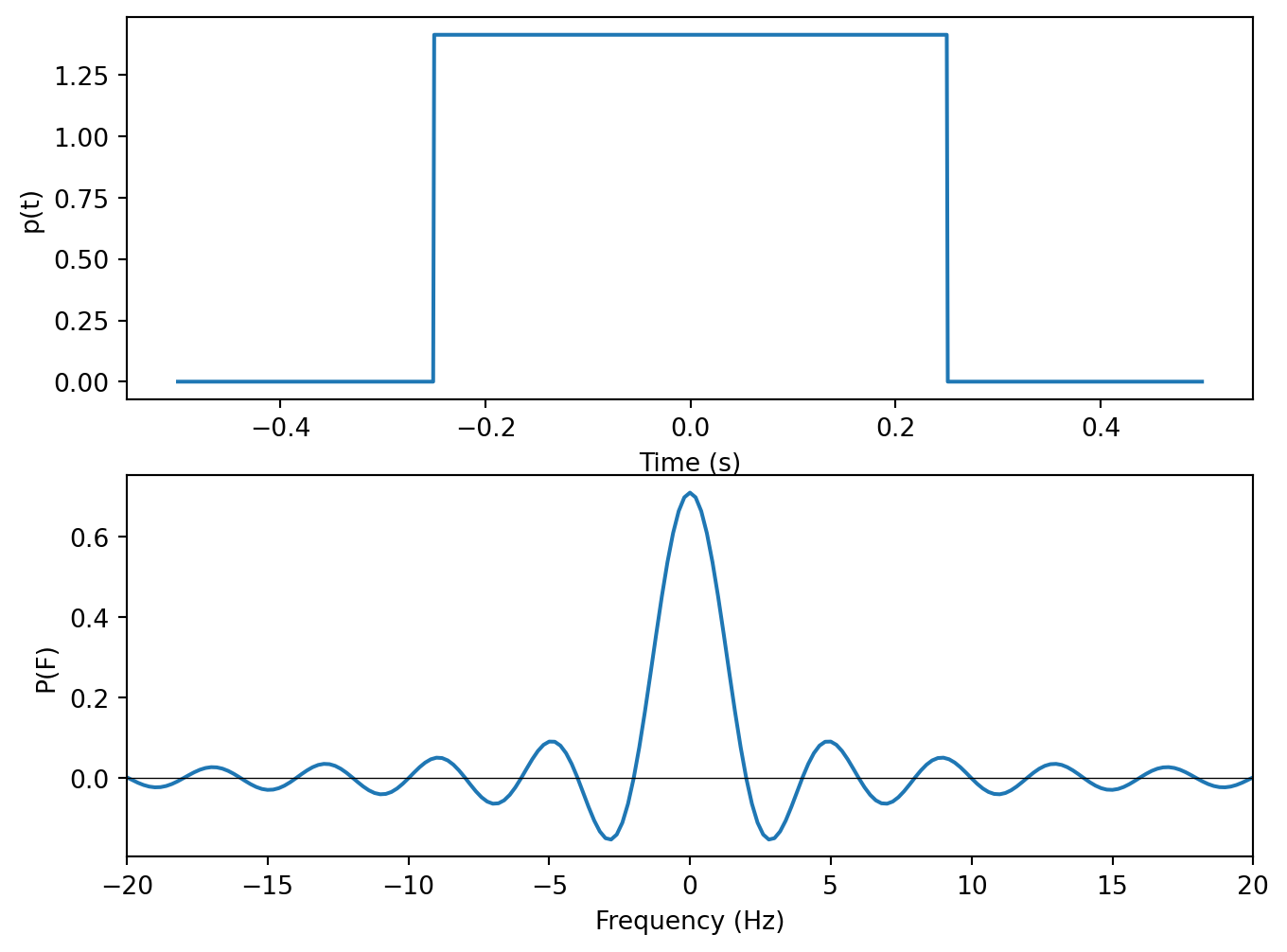
The rectangular pulse shape is very simple in the time domain. It is a pulse that remains high for some duration \(\beta T_s\) and then goes low. The height of the pulse is typically normalized so that the pulse has unit energy. \(\beta\) is called the duty cycle and indicates the ratio between how long the pulse is low and high. Therefore we can say that a pulse with \(\beta=1\) is always on (DC) while a pulse with \(\beta < 1\) will cycle between high and low. We call these two pulses return-to-zero (RTZ) and non-return-to-zero (NRZ) respectively. \(T_s\) is the period of the pulse.
In the frequency domain, the rectangular pulse looks like a sinc. Recall that the sinc extends infinitely along the x-axis, which in this case means that a rectangular pulse shape has an infinite bandwidth. It is for this reason that the rectangular pulse is not feasible in wireless communications. Spectrum space is heavily regulated across the world, which means that often only a narrow band will be assigned for a given purpose. A pulse shape suitable for wireless communications would have to fit into one of these narrow bands.
The rectangular pulse shape is often used in wireline communcations where there are no bandwidth limitations because the circuitry required to transmit and receive is very simple.
import matplotlib.pyplot as plt
import numpy as np

Ts = 1      # period of pulse

pad = 10000
sample_rate = .001  # sampling rate to simulate continuous time
n = int(Ts/sample_rate) * pad # increase length for better FT resolution
t = np.arange(n) * sample_rate - pad*Ts/2
h = 1/np.sqrt(Ts) * np.sinc(t/Ts)

f = np.fft.fftfreq(len(h), d=sample_rate)
f = np.fft.fftshift(f)

plt.figure(figsize=(8, 6))
plt.subplot(2, 1, 1)
plt.plot(t, h)
plt.xlim([-5*Ts,5*Ts])
plt.ylabel("p(t)")
plt.xlabel("Time (s)")
plt.axhline(0, color="k", linewidth=.5)

h = np.fft.ifftshift(h) # move t=0 to front of array and ensure h is symmetric for DFT
H = np.fft.fft(h) / (n/pad)
H = np.fft.fftshift(H) # shift DC to center

plt.subplot(2, 1, 2)
plt.plot(f, H.real)
plt.ylabel("P(F)")
plt.xlabel("Frequency (Hz)")
plt.xlim([-1/Ts,1/Ts])
plt.axhline(0, color="k", linewidth=.5)

plt.show()
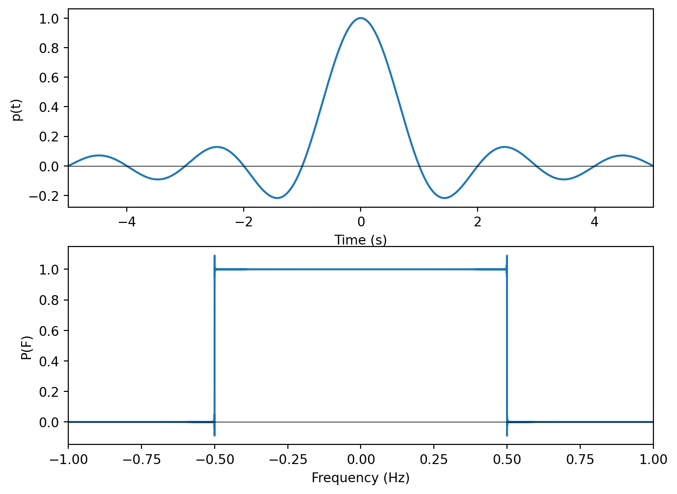
The sinc pulse shape is essentially the inverse of the rectangular pulse shape. It has an infinite duration in time, but a perfectly fixed bandwidth in frequency. Because it is impossible to construct a signal which is infinite in time, this pulse shape is not physically realizable. In practice, the pulse is truncated at some point in time which makes it possible to construct, but also increases the signal’s bandwidth.
import matplotlib.pyplot as plt
import numpy as np

plt.figure(figsize=(8, 6))
for a in np.linspace(0, 1, 5):
    Ts = 1      # period of pulse

    pad = 1000
    sample_rate = .001  # sampling rate to simulate continuous time
    n = int(Ts/sample_rate) * pad # increase length for better FT resolution
    t = np.arange(n) * sample_rate - pad*Ts/2
    empty = np.empty(n)
    empty[:] = np.nan
    h = 1/Ts * np.sinc(t/Ts) * np.divide(np.cos(np.pi*a*t/Ts), (1-(2*a*t/Ts)**2), out=empty, where=(1-(2*a*t/Ts)**2)!=0)

    f = np.fft.fftfreq(len(h), d=sample_rate)
    f = np.fft.fftshift(f)

    plt.subplot(2, 1, 1)
    line, = plt.plot(t, h)
    line.set_label(rf"$\alpha = {a}$")
    plt.legend()
    plt.xlim([-5*Ts,5*Ts])
    plt.ylabel("p(t)")
    plt.xlabel("Time (s)")
    plt.axhline(0, color="k", linewidth=.5)

    h = np.where(np.isnan(h), np.zeros_like(h), h)
    h = np.fft.ifftshift(h) # move t=0 to front of array and ensure h is symmetric for DFT
    H = np.fft.fft(h) / (n/pad)
    H = np.fft.fftshift(H) # shift DC to center

    plt.subplot(2, 1, 2)
    line, = plt.plot(f, H.real)
    line.set_label(rf"$\alpha = {a}$")
    plt.legend()
    plt.ylabel("P(F)")
    plt.xlabel("Frequency (Hz)")
    plt.xlim([-1/Ts,1/Ts])
    plt.axhline(0, color="k", linewidth=.5)

plt.show()
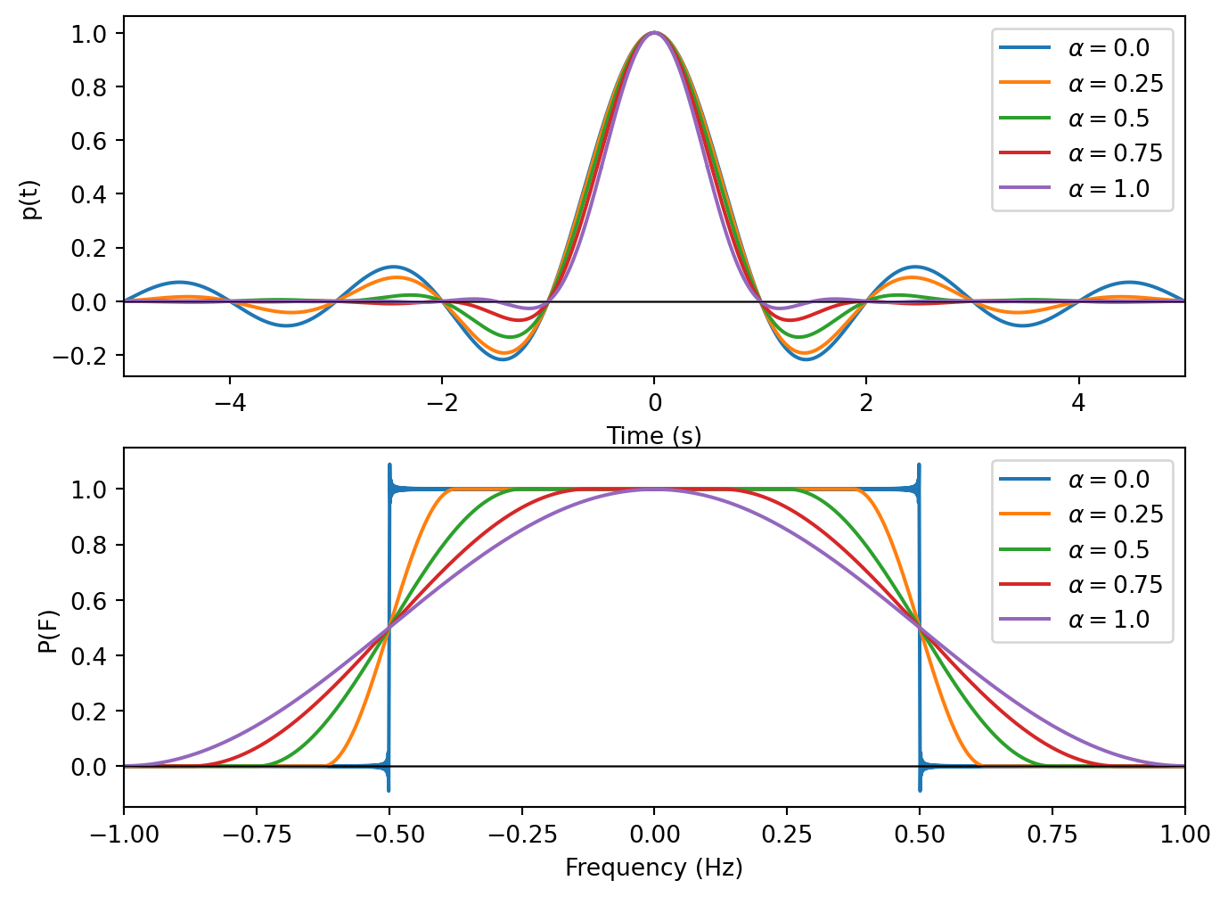
In most cases we strive to be somewhere in between the two extremes of the rectangular pulse and the sinc. The most commonly used pulse shape in this “in between” is the raised cosine pulse. The equation for the raised cosine pulse is rather involved, but the pulse can be practically characterized by a single parameter \(\alpha\), typically called excess bandwidth (or sometimes roll-off). \(\alpha\) is a number between \(0\) and \(1\), where \(\alpha = 0\) corresponds to a perfect sinc in the time domain and \(\alpha = 1\) corresponds to a cosine in the frequency domain.
The important thing to note is that for any \(\alpha\), the pulse is bandlimited. Increasing \(\alpha\), (i.e., excess bandwidth) leads to a pulse that decays to 0 in the time domain much faster than a sinc at the cost of slightly more bandwidth. Because the raised cosine decays significantly faster than a standard sinc (sinc decays as \(1 / t\) while the raised cosine decays as \(1 / t^3\)), truncation in the time domain causes much less distortion in the frequency domain when compared with a sinc.
Selecting the correct excess bandwidth for the pulse depends on the system parameters desired. Faster transmission of data requires the pulses to be shorter (which usually means a harsher truncation) and thus the bandwidth to be larger. On the other hand, signals which require a smaller bandwidth are better served with a smaller value of \(\alpha\) so that there is not as much distortion in the frequency domain.